What the Sampling Theorem Really Promises (and What It Doesn’t)

Chris Lomont, with Claude Fable 5.2

What this article is. The general-audience article in a pair on the sampling theorem: what the famous rule promises, what it quietly assumes, and what happens when the assumptions fail. For engineers, programmers and curious readers.

Related articles. Full treatment with mathematics and references: Where the Sampling Theorem Stops . Checklist: Best Practices and Gotchas . Companion topics: image resampling, dithering and quality metrics (summary ); color spaces and HDR (summary ).

This is the short version of the sampling theory notes; for how and why they were written, see the introduction to the main article .

Contents

• The famous rule
• Five things the rule quietly assumes
• A common myth
• Can we do better than “twice the highest frequency”?
• The catch
• Three questions to ask of any claim
• Practical rules that follow

The famous rule

Almost everything digital that touches the physical world (music, photos, video, radio, medical scans) starts by sampling: measuring a continuously varying quantity at regular instants and keeping only the list of measurements.

The sampling theorem says when that loses nothing. If a signal contains no frequencies above some limit, then measuring it more than twice per cycle of that highest frequency captures it completely; the original curve between the measurements can be rebuilt exactly. That is why CDs use 44,100 samples per second for sound that tops out near 20,000 cycles per second.

The rule is true. It is also a statement about an idealized world, and each of its idealizations fails in a specific, measurable way. Knowing how is the difference between using the rule and being surprised by it.

Five things the rule quietly assumes

1. That the signal really has a highest frequency. No real signal does. Anything that starts and stops, or has a sharp edge, contains some energy at every frequency. Frequencies above half the sampling rate do not vanish when sampled: they reappear disguised as lower ones. This is aliasing . It is why wagon wheels turn backward in films, why a striped shirt shimmers on video, and why a shrunken photo of a brick wall can show swirling patterns that were never there.

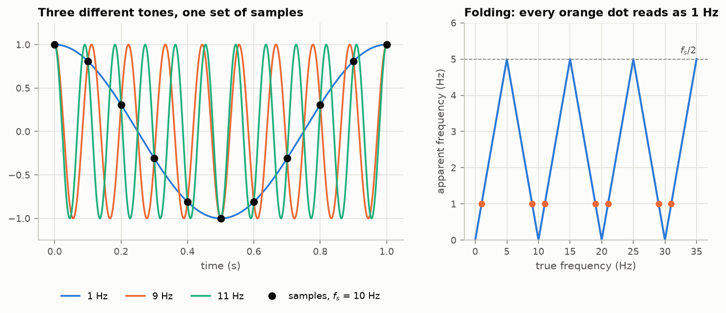
Three different tones that produce exactly the same samples. Once sampled, nothing can tell them apart.

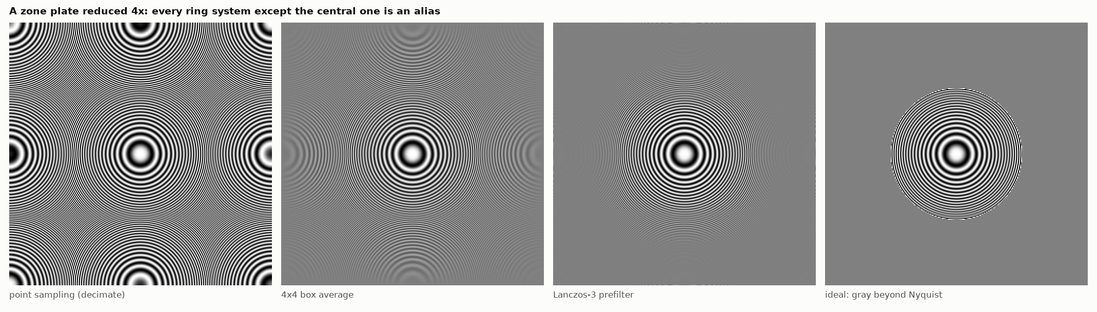
A pattern of ever-finer rings, shrunk to a quarter size. Simply dropping pixels (left) invents eight extra sets of rings. Blurring before shrinking (middle panels) removes most of them. The honest answer (right) is plain gray wherever the rings are too fine to show.

The cure is to blur before sampling, removing what cannot be represented. The blur is never perfect, so the practical question is never “is there aliasing?” but “how much, and does it matter?”

2. That the measurements are exact numbers. They are not; they are rounded to a fixed number of bits. The usual story is that rounding adds a faint hiss. That is only true when the signal is large and busy. For quiet or simple signals the rounding error is not hiss at all but distortion that follows the signal around.

The fix is one of the nicest surprises in engineering: add a little noise on purpose before rounding. This “dither ” turns the distortion into a steady, harmless hiss, and even lets signals smaller than one rounding step come through.

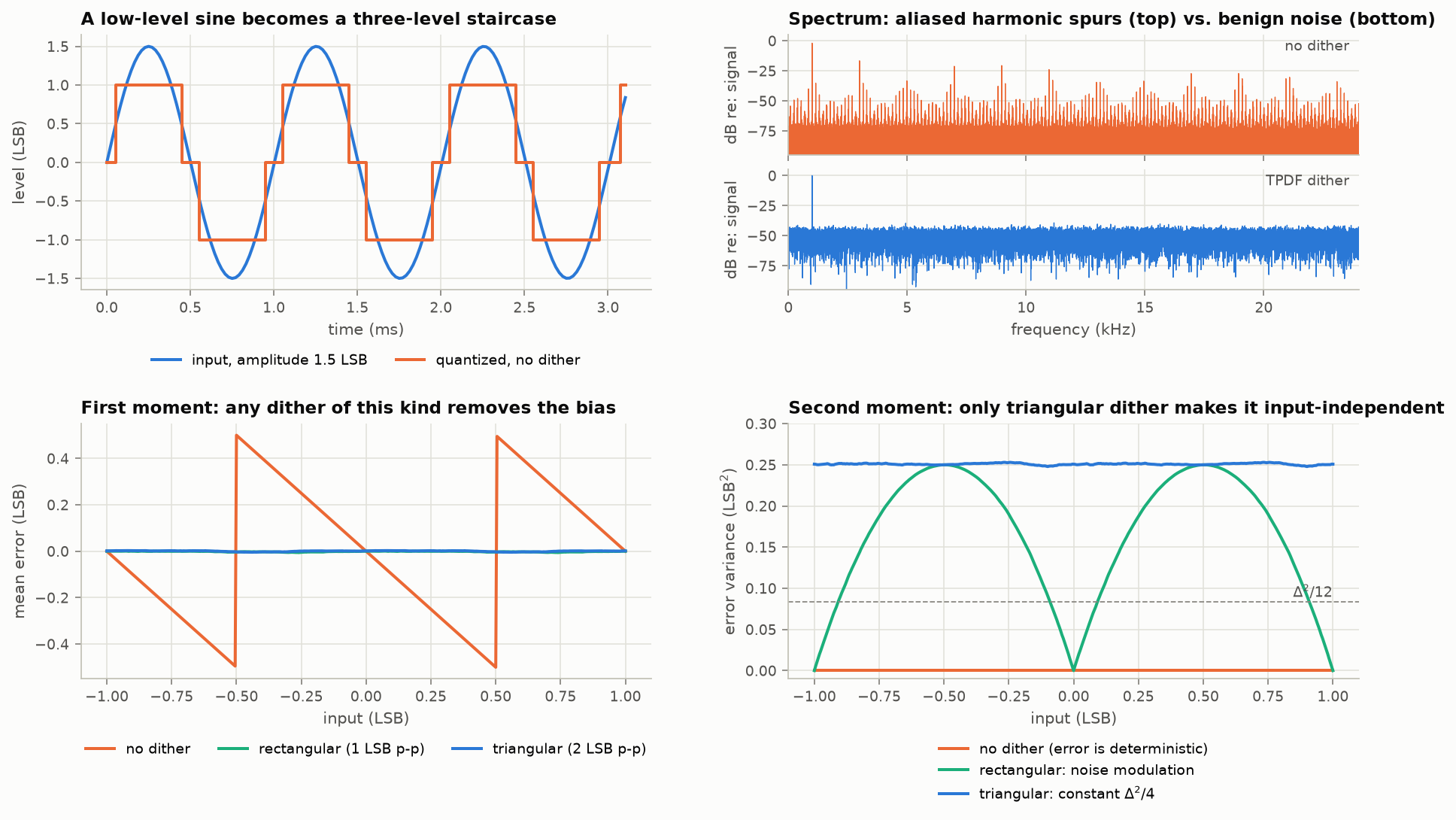
Top left: a quiet tone rounded to three levels. Top right: without dither, the result is full of false tones; with dither, it is the original tone plus a smooth noise floor.

There is a deeper point. With exact measurements, “how many samples?” is the whole question. With rounded ones, the real budget is bits, and bits can be spent on more samples or on finer rounding. Many modern converters take this to the limit: they measure with a single bit, millions of times per second, and get 24-bit quality by clever feedback.

3. That the measurements happen at exactly the right instants. Clocks wobble. A wobble of one trillionth of a second sounds negligible, but for a fast signal it limits accuracy to about 10 bits, no matter how many bits the converter advertises. At high frequencies, the clock matters more than the bit count.

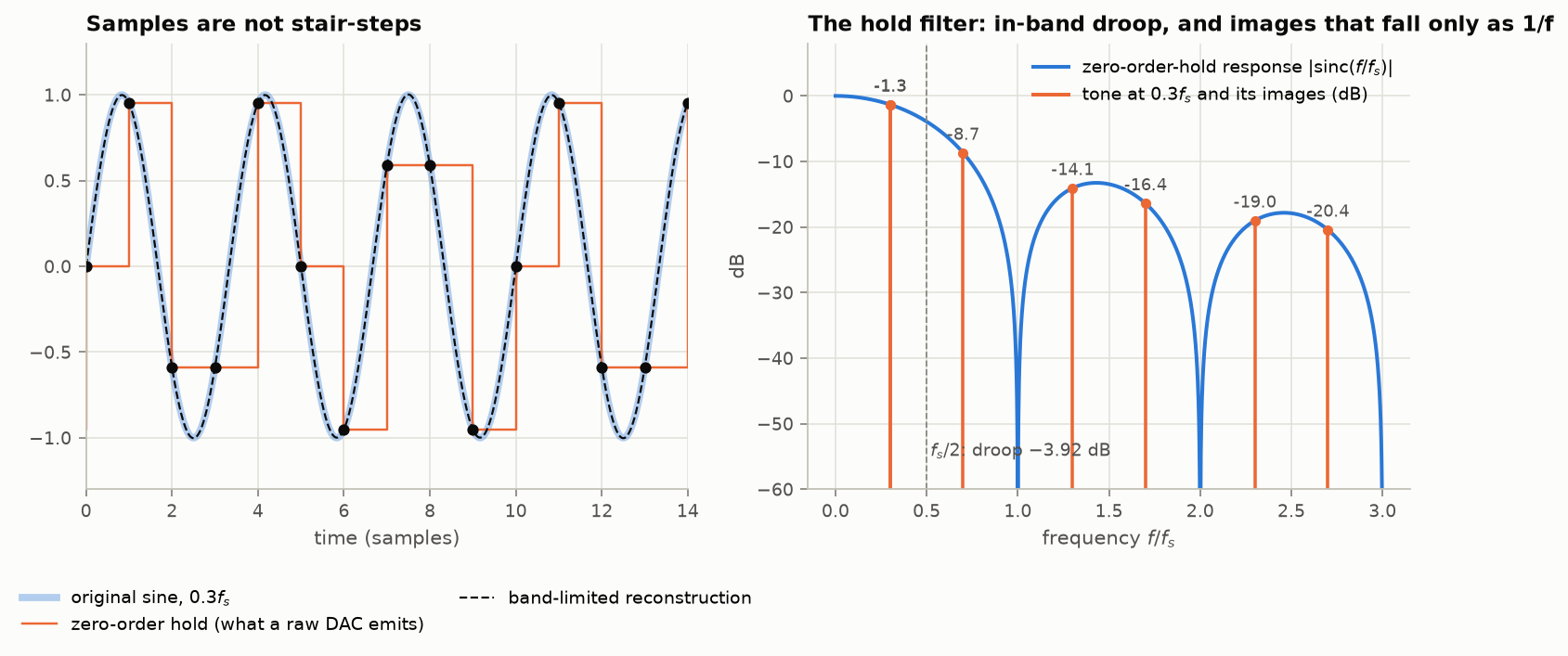
4. That you can rebuild the curve with a perfect filter. The exact rebuilding formula uses every sample, infinitely far in both directions. Real systems use a short approximation, and short approximations only work if you sample somewhat faster than the theoretical minimum. Sharp filters also “ring” near sudden changes, so designers trade sharpness against ringing against leftover aliasing. No choice wins on all three.

A related surprise: a digital recording whose samples never exceed the maximum can still produce an output that does, because the true curve can peak between samples.

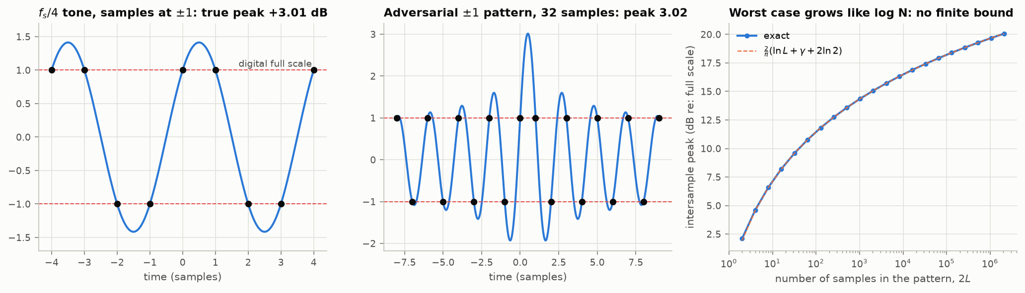
Left: every sample sits at the limit (dashed), yet the curve through them overshoots by 41%. Middle and right: a contrived pattern overshoots by 200%, and in principle there is no ceiling.

5. That the samples are evenly spaced and all present. Having enough samples on average is not enough. Samples bunched together, or a stretch of missing ones, can in theory be worked around, but the arithmetic amplifies the slightest noise enormously. “Possible in principle” and “works in practice” part company here, and they do so throughout this subject.

A common myth

Digital audio is often drawn as a staircase, suggesting that it is a crude, blocky version of the real thing. The staircase is an intermediate step inside the converter. After its output filter, what comes out is a smooth curve passing through every sample: for a signal within the frequency limit, the same curve that went in.

Can we do better than “twice the highest frequency”?

Yes, but not by cheating the rule. The rule is airtight for the kind of signal it describes. What has changed over the last few decades is the realization that “contains no high frequencies” is often the wrong description of real signals, and that a better description needs fewer numbers.

• Edges. A photograph is mostly smooth regions separated by sharp edges. Describing an edge with smooth waves takes a huge number of them, and they leave ripples. Wavelets , little localized waves of many sizes, describe the same edge with a handful of numbers. That is the idea behind JPEG 2000. Curvelets and shearlets go further by also being long and thin, so they can lie along a curved edge.

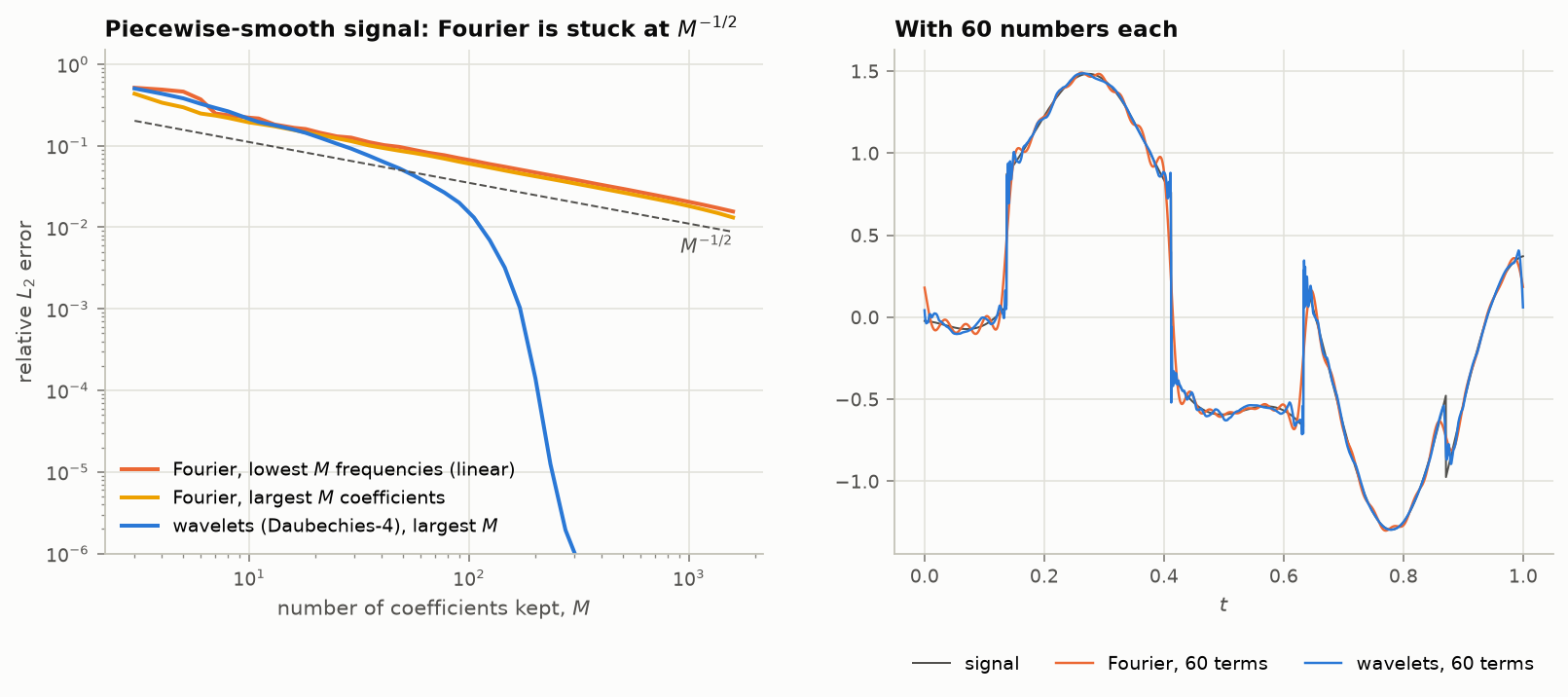
A signal with sudden jumps, described with 60 numbers. Classical waves (orange) ripple everywhere. Wavelets (blue) are wrong only right at the jumps.

• Mostly empty signals. If a signal is built from only a few ingredients out of many possible ones, a few measurements suffice, provided they are taken in a deliberately irregular pattern. This is compressed sensing ; it is used to shorten MRI scans.

• Signals defined by a few numbers. A train of sharp pulses is the opposite of a smooth signal, yet it is fully described by when each pulse happens and how big it is. Measure a blurred version just a few times and those numbers can be solved for exactly.

• Signals that overflow the sensor. A new kind of sensor “wraps around” instead of clipping, like an odometer. Sampled fast enough, the original can be unwrapped even when it is many times too large for the sensor.

In every case the count of measurements still matches the count of things you do not know. What changed is which things are counted.

The catch

Each of these methods leans on an assumption about the signal, and each breaks, sometimes abruptly, when the assumption is slightly off.

• Compressed sensing recovers a few pure tones perfectly from a quarter of the usual samples. Nudge the tones by a fortieth of a frequency step and the error jumps from one part in a trillion to five percent.
• Resolving two objects closer together than a lens “should” allow is possible, but the required measurement quality grows explosively with how much finer you want to see.
• Unwrapping an overflowing signal works perfectly on clean data and can fail completely with half a percent of noise.

Plain, old-fashioned sampling fails gently: sample a little too slowly and you get a little aliasing. Most of the alternatives fail suddenly.

Three questions to ask of any claim

When someone says a system “beats the Nyquist limit,” ask:

1. How many unknowns does their model of the signal really have? They cannot use fewer measurements than that.
2. How much does the method amplify noise? Exact on paper can be useless in practice.
3. What happens when the signal does not quite fit the model?

Practical rules that follow

• Sample comfortably faster than twice the highest frequency you care about; the margin is what makes practical filters possible.
• Always filter before you sample or shrink. Never shrink an image by just dropping pixels.
• When reducing bit depth, add dither.
• Judge a converter by its measured performance at your signal’s frequency, not by its nominal number of bits.
• Leave headroom: the true signal can exceed the largest sample.
• Any operation that distorts a signal (clipping, squaring, heavy compression) creates new high frequencies. Do it at a higher sampling rate, then filter and come back down.
• Be suspicious of your tools: a plotting program, an image viewer or a resizing library may itself be sampling carelessly, and the artifacts you see may be its own.