What the numbers in a picture mean, from the CIE observers to HDR formats, and how they go wrong. Four articles: expert notes with computed figures and references; a general-audience summary ; a guide to best practices, gotchas and recognizing errors ; and reference tables with formulas.

Color Spaces and HDR: Representations, Standards, Stops, and How They Fail

Chris Lomont, with Claude Fable 5.2

What this article is. The expert-level article in a pair on color representation and high dynamic range. It covers the CIE observers, where color arithmetic is and is not linear, transfer functions, what “stops” means, bit allocation and packing formats, gain maps, and how each of these fails, with computed figures and full references.

Related articles. General-audience version: What the Numbers in a Picture Really Mean . Lookup tables: Reference Tables . Symptom-first error guide: Best Practices and Gotchas . Companion topics: image resampling, dithering and quality metrics (summary ); sampling theory and where it stops (summary ).

Introduction

Here are notes I co-developed with Claude Fable 5.2 in October 2026 on how color and HDR are represented in pictures and video, and how those representations fail. They draw on about 70 standards, papers and books, including very recent results. Public PDFs are linked where possible; other references point to their sources.

I also wanted one place for the things that are usually scattered: the CIE observers, transfer functions, bit depths and packing formats, gain maps, and where displays are heading. The main idea that I push when talking about color to engineers is that the numbers representing a color need to keep track of the units those numbers represent, and this is often lost in many pieces of software. Another thing I wanted to chase down is how often different sources claim “Item X represents Y stops,” and often these claims differ significantly. This helps show why, and clean up some misconceptions. The same goes for “percent of gamut” claims.

Sections on recognizing errors by their look, on future directions, and on what is known and unknown close the notes.

I also made a simpler summary of these notes, a list of best practices and gotchas , and reference tables with formulas.

Contents

• Introduction
• 0. Scope
• 1. A pixel is a number without units
• 2. The observers: 1931, 1964, Judd–Vos, 2006, 2015
  • 2.1 What a standard observer is
  • 2.2 Why it did not matter, and why it does now
• 3. Chromaticity, gamuts, and why a triangle is the wrong picture
• 4. Where color is additive, and where it is not
• 5. Transfer functions
  • 5.1 The SDR family, and three persistent confusions
  • 5.2 PQ (SMPTE ST 2084, BT.2100)
  • 5.3 HLG (BT.2100)
  • 5.4 Reference white, and what “1.0” means
  • 5.5 Scene-referred, display-referred, and the OOTF
• 6. Stops: one ruler
  • 6.1 Encodings (quantities C and D)
  • 6.2 Sensors (quantity B)
  • 6.3 Log encodings (quantity E)
  • 6.4 Film, displays and eyes
• 7. Bits: where the codes go, and what fits in what
  • 7.1 Packing problems
  • 7.2 Round trips
  • 7.3 Banding and dither
  • 7.4 Rounding rules: bytes, floats and bit-depth changes
  • 7.5 HDR bit depth, measured one way
• 8. A color float: design study
  • 8.1 What color needs from a float
  • 8.2 Uniform-mantissa unsigned floats, exmy
  • 8.3 Two improvements specific to color
  • 8.4 Candidate layouts
• 9. Luma, chroma and subsampling
  • 9.1 What $Y'C_bC_r$ is
  • 9.2 The J:a:b notation
• 10. Arithmetic in the right space
  • 10.1 Tone mapping and the hue of highlights
  • 10.2 Gamut mapping
• 11. Gain maps and Ultra HDR
  • 11.1 The mechanism
  • 11.2 Failure modes
  • 11.3 Making gain maps: details that decide the result
• 12. Recognizing errors by their look
  • 12.1 Constants and tags that circulate wrongly
• 13. Directions
  • 13.1 More than three primaries
  • 13.2 Other directions
• 14. Known, unknown, contested
• 15. Sources

0. Scope

This article concentrates on the parts of color and HDR practice where the numbers are most often misread:

• the CIE observers from 1931 to 2015, with a computed demonstration of what narrowband primaries do to them (§2 );
• where color arithmetic is linear and where it is not, including brightness (§4 );
• a single ruler for “stops”, with every common definition applied to the same signals (§6 );
• bit allocation, packing formats, and a worked design study for a “color float” (§7 , §8 );
• gain maps and their failure modes, simulated (§11);
• multi-primary displays and other directions (§13 );
• what is known, unknown and contested (§14 ).

Three conventions are used throughout. Linear means proportional to light (radiance or luminance). A prime, as in $R'$ or $Y'$, means a nonlinearly encoded value. Luminance is in cd/m² (“nits”). Claims are marked as follows: [std] read in a standard or specification; [calc] computed for this article [Code]; [2nd] from a secondary source and not checked against the primary; [prior] a calculation or measurement made before this article and outside its figures, not rerun for it.

---

1. A pixel is a number without units

A triple such as (0.5, 0.2, 0.1) means nothing until seven things are declared. Almost every color bug is one of them lost, guessed or mixed.

Tag	Question it answers	Typical values
Primaries	Which three lights?	BT.709 , Display P3, BT.2020 , ACES AP0/AP1
White point	Which light is “equal RGB”?	D65 , D60, DCI white, D50
Transfer function	How do numbers map to light?	sRGB , BT.1886 (γ 2.4), PQ, HLG , linear, camera log
Range	Which codes are black and white?	full (0–255), narrow (16–235)
Matrix	Is it RGB or a luma/chroma form, and which?	identity, BT.601 , BT.709, BT.2020 NCL, ICtCp
Reference white	What does 1.0 (or 100%) mean in cd/m²?	80, 100, 203, “diffuse white”, “1 nit”
Observer	Whose eyes define the match?	CIE 1931 2° (nearly always, silently)

ITU-T H.273 gives the first five numeric code points (CICP ), and those four numbers (primaries, transfer, matrix, range flag) are what video streams, AVIF, HEIF and now PNG carry [std]. The last two tags have no code point. Reference white is a convention that differs by industry, and the observer is assumed.

The thesis in one line: a pixel value is a number in an undeclared unit system.

---

2. The observers: 1931, 1964, Judd–Vos, 2006, 2015

2.1 What a standard observer is

Human color matching is linear to a good approximation (Grassmann ’s laws). Three numbers therefore summarize any spectrum $S(\lambda)$:

$$X = k\!\int S(\lambda)\,\bar x(\lambda)\,d\lambda,\qquad Y = k\!\int S(\lambda)\,\bar y(\lambda)\,d\lambda,\qquad Z = k\!\int S(\lambda)\,\bar z(\lambda)\,d\lambda .$$

The color-matching functions (CMFs) $\bar x,\bar y,\bar z$ are a linear transform of the three cone sensitivities, averaged over a group of people and tied to a field size. Two spectra with equal XYZ are metamers: they match for that average observer. Every RGB space, every display calibration and every color-difference formula is built on a choice of CMFs.

Observer	Basis	Field	Status
CIE 1931	Wright and Guild matches, 17 observers in total, forced through the 1924 $V(\lambda)$	2°	The observer in every imaging standard
Judd 1951, Vos 1978	Corrections to the 1931 functions below about 460 nm	2°	Used in vision science; never adopted for imaging
CIE 1964	Stiles and Burch, about 50 observers	10°	Standard for fields larger than 4°; used in color-difference work
CIE 170-1:2006	Cone fundamentals (LMS) from Stockman and Sharpe, parameterized by field size (1–10°) and age (20–80)	any	A physiological model, not a single table
CIE 170-2:2015	Cone-fundamental-based $V_F(\lambda)$ and tristimulus functions $\bar x_F,\bar y_F,\bar z_F$ for 2° and 10°, 32-year-old observer; MacLeod–Boynton diagram	2°, 10°	Published, but “seen limited use in practical applications” (Royer et al. 2023) [std]

“CIE 2006” and “CIE 2015” are therefore the same physiological model: 2006 gave the cone fundamentals, 2015 turned them into XYZ-like functions that can replace the 1931 ones. CIE 015:2018 still recommends 1931 for fields of 1–4° and 1964 above 4°, and every derived tool (CIELAB , ΔE2000, correlated color temperature, CIECAM16) is defined on those two [prior, from CIE 015:2018]. The web pass found no display or video standard that uses the 2015 functions [2nd].

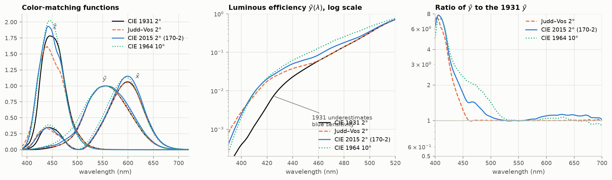
Figure 1. Left: four sets of color-matching functions. Middle: the luminous-efficiency function on a log scale; the 1931 curve is too low in the blue. Right: ratio to the 1931 curve. Below 450 nm the later observers are 1.5 to 8 times more sensitive than 1931 says. Data: CVRL tables.

2.2 Why it did not matter, and why it does now

The 1931 error is confined to short wavelengths. A CRT phosphor or a filtered white LED spreads its blue over 50 nm or more, and the error averages out. A laser or a narrow quantum-dot or OLED emitter puts all of its blue power at one wavelength, where the observers disagree most.

Figure 2 computes this. Four displays are each adjusted so that the 1931 observer sees exactly the same white as a 6504 K blackbody. The same spectra are then evaluated with other observers.

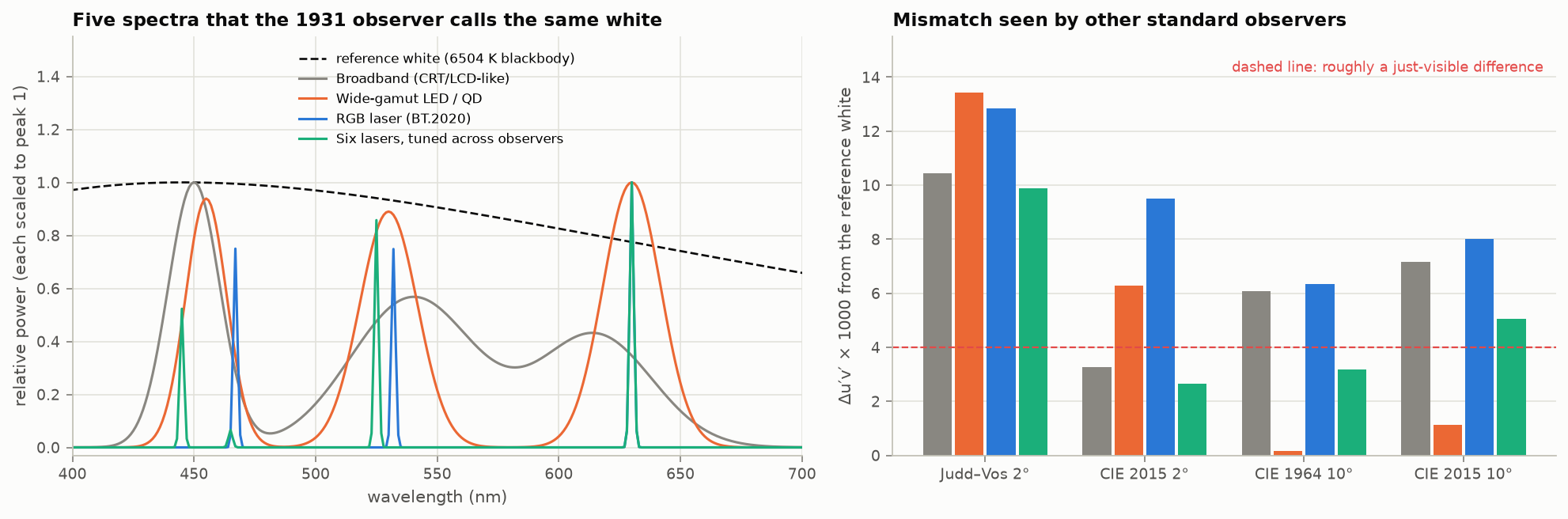
Figure 2. Left: four display whites and the reference, all identical to the 1931 observer. Right: how far each display white lands from the reference for four other standard observers, in $\Delta u'v'$. A value near 0.004 is commonly taken as visible. [calc]

Three things to take from it [calc]:

• For the CIE 2015 2° observer, the broadband display misses by $\Delta u'v' \approx 0.003$, the wide-gamut LED by 0.006 and the three-laser display by 0.0095. Narrower primaries give larger disagreement.
• The answer depends on which alternative observer is used, and the ordering is not always the same (the LED case happens to agree with the 10° observers). No single replacement observer fixes the problem; real people scatter around all of them.
• Six lasers with weights chosen to satisfy three observers at once cut the laser mismatch by half to two-thirds. Extra primaries buy metameric freedom, not just gamut (§13 ).

This is the origin of the “my calibrated OLED does not match my calibrated LCD” complaint, and of the practice of applying a white-point offset to OLED and laser reference monitors (often called a Judd or Judd–Vos offset). The offset is a patch for the average viewer. It does nothing for the spread between individuals, which recent modeling puts as substantial for narrowband displays and worst for older lenses and anomalous cone pigments (Rider, Frith and Stockman 2026 [2nd]). The model of Asano, Fairchild and Blondé (2016) simulates the spread among color-normal observers by adding eight physiological parameters (lens and macular pigment density, cone optical densities, cone peak shifts) to the CIE 2006 observer; it does not itself address narrowband displays or anomalous pigments. A 2026 study with 30 observers and 9,300 matches to 56 near-white stimuli found variability markedly larger for a laser projector, then an RGB mini-LED display, than for an LCD, and traced it to the spectral shape of the primaries, with gamut area having little effect (Li and co-authors 2026 [abstract only]). Measured color matches of 51 young adults agree with the CIE 2006 observer except for a 3 nm shift of the M-cone pigment toward longer wavelengths and a slightly denser macular pigment in the 2° field; differences between observers in the 10° matches averaged about 4 ΔE00 in RGB terms, against about 1 for one observer repeating a match (Shi and co-authors 2024 [pp. 1, 7–8]). For laser cinema, maps of observer metamerism show that “achromatic highlights could be particularly prone to disagreements between observers” (Trumpy and co-authors 2023 [read online]).

Practical rule. Two displays with different emission spectra cannot be made to match for everyone by colorimetry. State the observer when reporting a match, and expect a few ΔE of disagreement between people on wide-gamut displays.

---

3. Chromaticity, gamuts, and why a triangle is the wrong picture

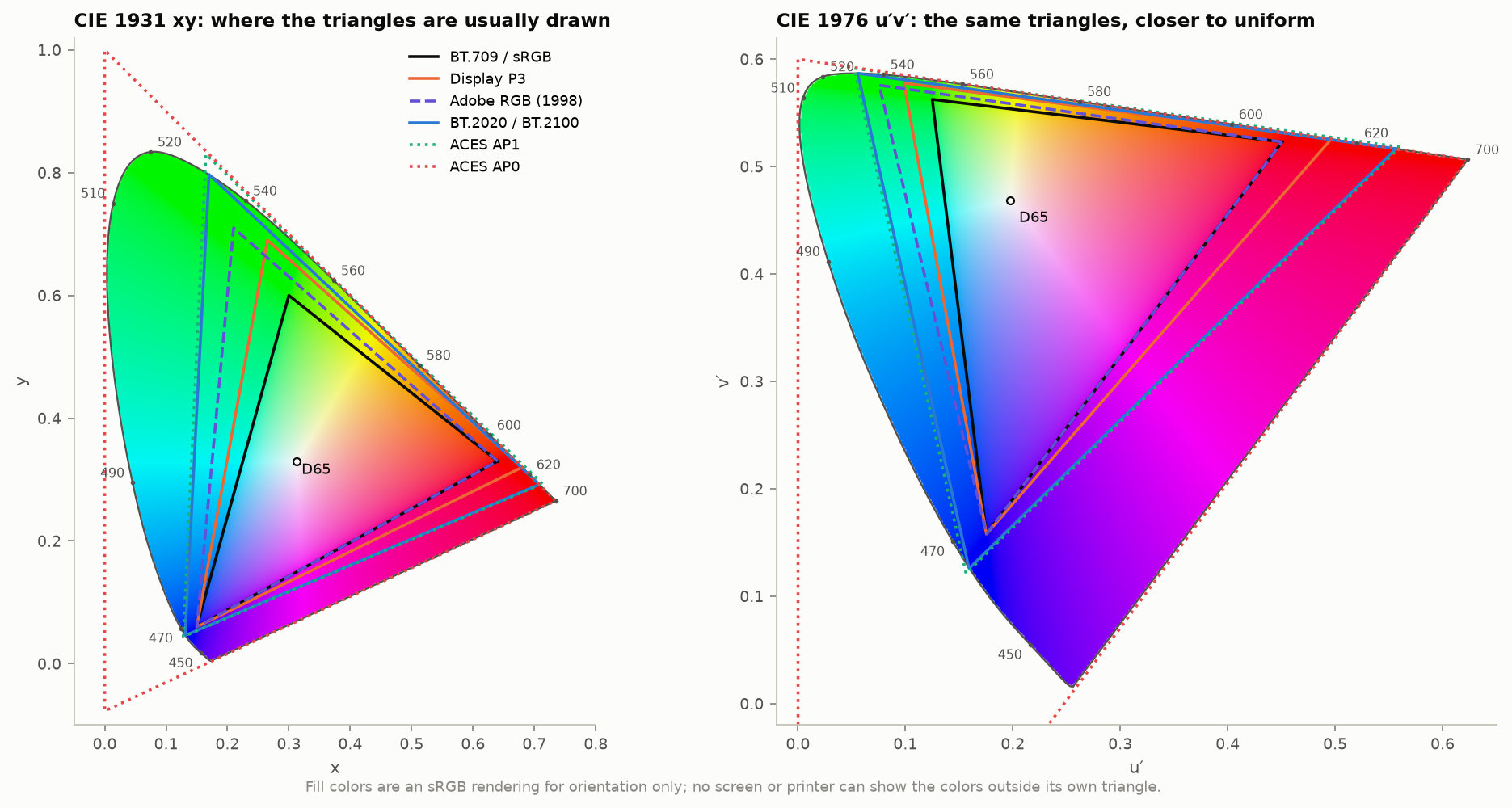
Figure 3. Common RGB primaries in the 1931 xy diagram and in the 1976 u′v′ diagram. The same triangles look very different: xy exaggerates green area.

Facts worth having at hand [calc]:

Space	Share of spectral locus area, xy	Share, u′v′
BT.709 / sRGB	34%	33%
Display P3	46%	42%
Adobe RGB (1998)	45%	39%
BT.2020	63%	57%
ACES AP1	67%	59%

“Covers 90% of BT.2020” therefore needs three qualifiers: which diagram (xy or u′v′), whether it is area coverage (intersection) or area ratio (which can exceed 100% while missing part of the target), and at what luminance. Reviewer measurements of 2025–2026 RGB-backlit televisions give 87–93% of BT.2020; claims of 100% or more are area ratios or marketing [2nd].

BT.2020’s primaries are spectral: 630, 532 and 467 nm. Only lasers reach them exactly. ACES AP0 encloses the whole locus by using primaries that are not physical colors, which is fine for storage and wrong for arithmetic (negative or absurd values under blending and grading), hence AP1 as the working space.

A gamut is a volume

The triangle shows which chromaticities a display can make at some luminance. At high luminance the set shrinks toward white, because a saturated color uses only one or two of the three emitters.

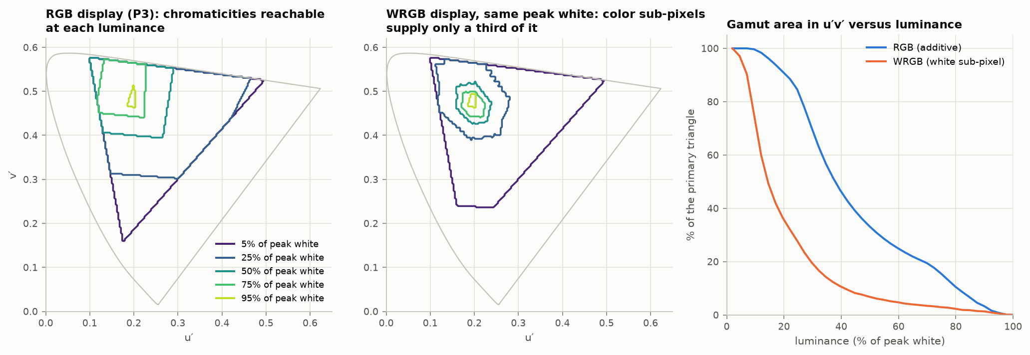
Figure 4. Left: chromaticities a P3 RGB display can show at five luminance levels. Middle: the same for a display that gets two-thirds of its peak white from a white sub-pixel. Right: gamut area against luminance. [calc]

For an ideal RGB display, the full triangle is available only below about 7% of peak white (the luminance of the blue primary). At half of peak white, about a third of the triangle remains. A display that adds a white sub-pixel (WRGB OLED, RGBW LCD, projectors with a white segment) loses color faster still: its saturated colors are capped at the luminance of the color sub-pixels alone. This is why the industry moved from “gamut area” to color volume, and why two televisions with the same peak nits and the same triangle can look very different on a bright red.

---

4. Where color is additive, and where it is not

“Colors are not additive at higher brightness” bundles four separate effects. It helps to keep them apart.

4.1 What is additive. Light is. If spectrum A has tristimulus values $T_A$ and B has $T_B$, the mixture has $T_A+T_B$, at any level a display can produce. Linear RGB arithmetic (blending, filtering, resizing) is exact physics. This holds from mesopic levels up to the point where photopigment bleaching changes the cone sensitivities, several thousand trolands and up, beyond most displays today.

4.2 Encoded values are not. Adding or averaging $R'G'B'$ values is not adding light. Figure 15 (§10 ) shows the visible result.

4.3 Brightness is not luminance. Luminance $Y$ is additive by construction (Abney’s law) because it is defined by flicker photometry , which isolates one visual pathway. Brightness, what a steady patch looks like, also draws on the chromatic pathways. At equal luminance a saturated color looks brighter than a gray: the Helmholtz–Kohlrausch (H–K) effect.

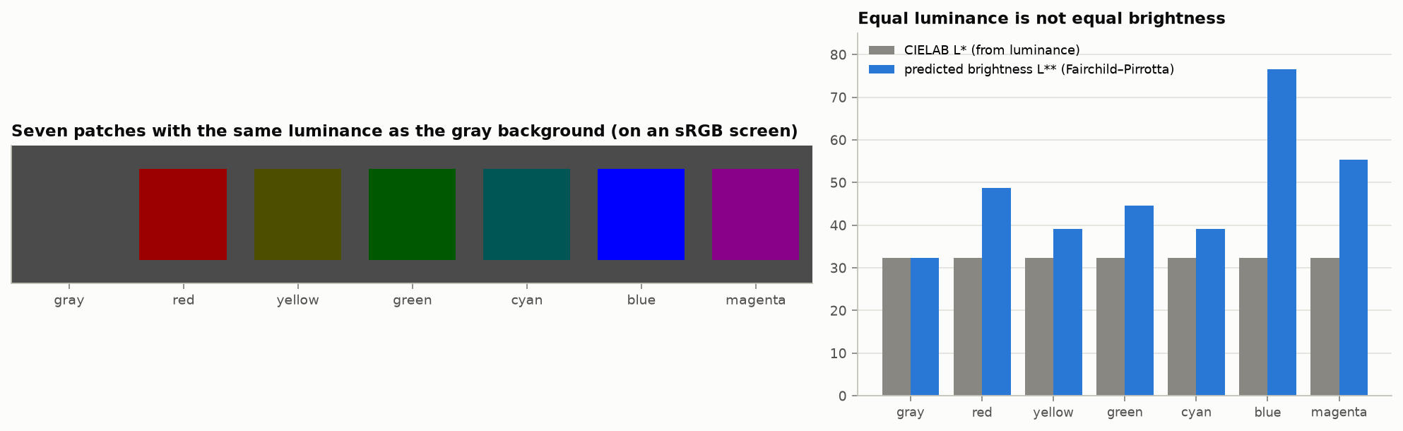
Figure 5. Left: seven patches with the same luminance as the background. On a calibrated sRGB screen the blue, magenta and red look clearly brighter than the gray, which should be nearly invisible. Right: CIELAB lightness (equal for all) against the Fairchild–Pirrotta brightness prediction. The blue value extrapolates the model well beyond the chroma range it was fitted on and should be read as “large”, not as a measurement. [calc]

The form of the Fairchild–Pirrotta predictor, $L^{\ast\ast}=L^{\ast}+f_2(L^{\ast})\,f_1(h_{ab})\,C^{\ast}_{ab}$, was checked against Fairchild’s book Color Appearance Models (2nd ed., eq. 6.3). The book does not print the two functions. The ones used for the figure, $f_2=2.5-0.025\,L^{\ast}$ and $f_1=0.116\,\left|\sin\frac{h_{ab}-90^\circ}{2}\right|+0.085$, are from memory, and a targeted search found no free source that prints them.

Consequences:

• Nits do not rank perceived brightness across colors. A 500 cd/m² saturated red highlight looks brighter than a 500 cd/m² white. Factors of 2 to 10 in equivalent luminance are reported for laser primaries [2nd]; a 2023 brightness-matching study on a laser projector (16 observers, 30 stimuli, mean variation between observers 15.9%) found that no existing appearance or equivalent-luminance model performed acceptably “due to a severe underestimation of the H-K effect”, and fitted a correction to CAM16 lightness, $J_{HK}=J+(1.52-0.013J)\,\big(0.65+0.11\,\tfrac{1-\sin h}{2}\big)\,C^{0.867}$ (Zhu and co-authors 2023 [read online]).
• Luma, $Y$, CIELAB $L^{\ast}$ and the $I$ of ICtCp carry no H–K term. Any tone mapper that holds one of them fixed while changing saturation changes apparent brightness.
• Brightness is not additive: two lights that each match a reference in brightness do not, when mixed, match twice the reference.

4.4 Appearance changes with level. With chromaticity fixed, raising luminance makes colors look more colorful (Hunt effect ) and raises apparent contrast (Stevens effect). Hue shifts with intensity (Bezold–Brücke ) and with added white (Abney effect , the reason a blue-to-white ramp in CIELAB turns purple; Figure 15). An image mastered at 1000 cd/m² and shown at 200 with the same chromaticities looks flatter and less saturated. This is why HLG applies a system gamma that grows with display peak (§5 ) and why “preserve chromaticity” is not the same as “preserve appearance”. Current appearance models disagree with each other at HDR levels; a comparison of models gives factors of 1.2 to 1.9 between them for the Hunt effect at 10,000 cd/m² [prior, computed].

4.5 Devices are not additive either.

• White sub-pixels (§3 ): $W \ne R+G+B$ in luminance.
• Power limiting: OLED and mini-LED sets reduce luminance as the bright area grows. Full-field white is roughly 25–60% of the small-patch peak [prior], so the same code value gives different light depending on the rest of the picture.
• Local dimming: a pixel’s black level depends on its neighbors.
• Crosstalk and color shift with drive level in OLED and LCD.

Each of these breaks the assumption behind a 3×3 matrix plus three 1-D curves, which is the model inside every ICC matrix profile and every simple display calibration.

4.6 CIELAB and ΔE need a white, and for displays it is not the peak. CIELAB normalizes by a reference white $Y_n$. For display light the CIE’s rule is to use the diffuse white the image simulates (203 cd/m² under BT.2408), not the display’s peak [std, CIE 015:2018]. Getting this wrong is easy to recognize. A 203 cd/m² diffuse white has $L^{\ast}=100$ when normalized correctly, 52 when normalized to a 1000 cd/m² peak, and 16 when normalized to 10,000. Color differences shrink with it, by factors of 0.59 and 0.27, so a difference of 2 reads as 1.2 or 0.55 and every tolerance stops meaning what it did [calc]. Highlights then have $L^{\ast}$ above 100, which is expected. Two related cautions: a Lab value or a ΔE without its illuminant and observer is not a measurement (the same red sample moves about 16 ΔE between illuminant A with the 2° observer and D65 with the 10° observer), and CIEDE2000 is specified for the 10° observer and small differences but is routinely applied to 2° data and large ones [std].

---

5. Transfer functions

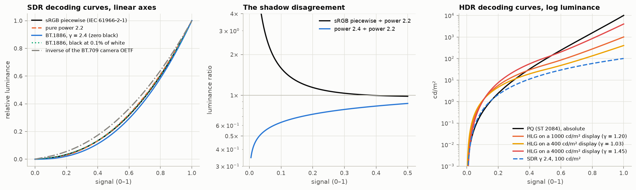
Figure 6. Left: SDR decoding curves. Middle: ratio of two of them to a pure 2.2 power; they agree in the midtones and differ by 2× or more in deep shadows. Right: PQ, HLG on three displays, and SDR on a log luminance axis.

5.1 The SDR family, and three persistent confusions

• sRGB encoding is piecewise: a linear toe of slope 12.92 joined to a 2.4 power with offset 0.055. The effective exponent is about 2.2.
• The sRGB display. Three different curves get called “the sRGB curve”. The encoding is the piecewise function above. The reference display in the 1997 committee draft is modeled as $((V'+0.055)/1.055)^{2.4}$ with no linear toe. And a pure 2.2 power is what the documents say the whole thing closely fits. The toe-less display model differs from the piecewise decode only for codes 0 to 9 at 8 bits (about three times more light at code 1). A pure 2.2 power differs from the piecewise decode by a factor of 8.7 in light at code 5, 3.8 at code 10, 1.9 at code 20 and 1.15 at code 50 [calc; for the draft, not the final 1999 text]. Which one to invert depends on the task: decode a file with the piecewise function; simulate or calibrate a display with whichever curve that display follows. The argument over which a display should follow is unresolved; reference monitors from some vendors ship piecewise, many consumer panels behave as 2.2 [2nd]. Symptom of a mismatch: shadows that are too light or crushed after an otherwise correct pipeline. A second search did not settle it. The 1996 W3C proposal says the piecewise equations were chosen to “closely fit a straightforward gamma 2.2 curve with an slight offset”; the technical secretary of the responsible IEC group is reported as saying the sRGB EOTF is unambiguously piecewise; and the author of the most careful public review concludes that the standard “lacks the clarity” for a definitive answer and recommends piecewise as a calibration target (all second-hand; the IEC text is paid and was not read) [2nd].
• BT.709 is a camera curve, not a display curve. Its OETF (exponent 0.45, linear toe 4.5) is not the inverse of the display. The display is BT.1886: a 2.4 power with a black-level term [std]. The mismatch is deliberate: the end-to-end exponent of about 1.2 compensates for a dim viewing surround. Decoding video with the inverse BT.709 OETF gives a washed-out picture.

$$L = a\,\max(V+b,\,0)^{2.4},\quad a=\left(L_W^{1/2.4}-L_B^{1/2.4}\right)^{2.4},\quad b=\frac{L_B^{1/2.4}}{L_W^{1/2.4}-L_B^{1/2.4}}\qquad\text{(BT.1886)}$$

5.2 PQ (SMPTE ST 2084, BT.2100)

PQ maps a signal $E'\in[0,1]$ to absolute display luminance up to 10,000 cd/m²:

$$L = 10000\left(\frac{\max\!\left(E'^{1/m_2}-c_1,\,0\right)}{c_2-c_3\,E'^{1/m_2}}\right)^{1/m_1},$$

with $m_1 = 0.1593$, $m_2 = 78.84$, $c_1 = 0.8359$, $c_2 = 18.85$, $c_3 = 18.69$. It was built by integrating the Barten threshold model so that each code step is about the same fraction of a just-visible difference (§7 ). Useful anchors [calc]:

Luminance (cd/m²)	0.005	0.1	1	10	100	203	1000	4000	10,000
PQ signal	0.015	0.062	0.150	0.300	0.508	0.581	0.752	0.903	1.000
10-bit narrow code	77	119	195	327	509	573	723	855	940

Half of the code range lies below 100 cd/m². “PQ is absolute” is true of the signal and false of most displays, which tone-map anything above their own peak and dim large bright areas.

PQ landmarks, exactly. Round numbers quoted for PQ are often wrong enough to break a test. A signal of 0.5 is 92.2 cd/m², not 100. A signal of 0.9 is 3906, not 4000. 203 cd/m² is signal 0.5807, 10-bit code 573 in narrow range and 594 in full range; “58%” decodes to 201.7. Test vectors built from the rounded landmarks are off by up to 8% [calc].

5.3 HLG (BT.2100)

HLG is scene-referred and relative: a square-root segment below 1/12 of peak scene light and a log segment above. The display applies a system gamma to luminance that depends on its peak, $\gamma = 1.2 + 0.42\log_{10}(L_W/1000)$ [std]. The same signal is therefore shown at different luminances on different displays by design. The 75% signal is reference white: 203 cd/m² on a 1000 cd/m² display [calc], and about 101 to 343 cd/m² on displays of 400 to 2000 cd/m² [calc; BT.2408].

HLG details that cause errors.

• Two normalizations. BT.2100 writes the OETF for scene light in [0, 1], with the breakpoint at 1/12. The original ARIB and BBC form uses [0, 12]. Mixing them is a factor of 12. Feed a 1 into the library: the answer is 1.0 in the first form and 0.5 in the second [std].
• Two gamma formulas. $\gamma=1.2+0.42\log_{10}(L_W/1000)$ is the BT.2100 formula for the usual production range of 400 to 2000 cd/m². Outside that range BT.2100 gives $\gamma=1.2\cdot1.111^{\log_2(L_W/1000)}$. At 4000 cd/m² the two give 1.453 and 1.481, and reference white lands at 581 or 559 cd/m² [std; calc].
• Reference white as light. The 75% signal comes out at $L_W\cdot0.265^{\gamma}$: 101, 203 and 343 cd/m² on 400, 1000 and 2000 cd/m² displays [calc].
• Full range. BT.2408 says full-range coding “should not be used” for HLG production. There is no room for filter overshoot, and clipping distorts [std].
• Tagging is not converting. Setting the transfer-characteristics tag to HLG on a stream labels it. Unless a conversion step runs, the pixels are unchanged. Test: encode a linear ramp, decode it, and compare with the HLG curve.

5.4 Reference white, and what “1.0” means

BT.2408 sets HDR reference white (a 100% diffuse white card, also graphics white) at 58% PQ or 75% HLG, which is 203 cd/m² on the reference display [std]. It is a signal level. Other conventions for linear 1.0 in floating point:

Convention	Linear 1.0 means
scRGB , Windows	80 cd/m²
BT.2100 display-referred float (Table 10)	1 cd/m²
Scene-referred (ACES, OpenEXR practice)	diffuse white, with 0.18 mid gray
Apple EDR, gain maps	SDR white, whatever the screen currently shows it at
BT.2408 practice	203 cd/m²

A half-float buffer handed between two systems that disagree here is off by a factor of 80, 203 or more, with no error raised.

Headroom on phones and laptops. Two operating systems now expose HDR headroom to applications. Apple’s extended dynamic range takes SDR reference white as 1.0 and reports how many times brighter the brightest pixels can currently be; the value changes with the brightness setting. Android reports the ratio of the HDR peak to the SDR white point, and dims SDR content as HDR brightness rises [web, developer documentation]. In both, headroom is a moving quantity, which is why a gain map’s rendering changes with screen brightness (§11).

5.5 Scene-referred, display-referred, and the OOTF

The opto-optical transfer function is the intended difference between scene light and display light: partly a contrast adjustment for the viewing surround, partly artistic rendering. PQ systems put it in the camera or grade, HLG puts it in the display. Camera log curves (LogC, S-Log, V-Log) and ACES are scene-referred and carry no rendering at all; viewed directly they look flat and gray. Converting between HDR systems without accounting for where the OOTF lives is a common source of “correct math, wrong picture”.

Where the OOTF lives, and how big it is.

System	Where the rendering intent is applied	End-to-end exponent
SDR television	Split: camera curve of about 1/1.95 effective, display 2.4	about 1.2
PQ	In production (the reference OOTF), so the signal is display light	about 1.2 at the reference display
HLG	In the display, from its peak and surround	1.2 at 1000 cd/m², rising with peak
sRGB in a 64 lux office	Display	about 1.1
Cinema, dark surround	Print and projection	1.5 to 1.8

Collected values [2nd]. Brighter surrounds want a lower exponent; BT.2390 gives a correction of about −0.076 per decade of surround luminance for HLG. Tests at two broadcasters gave optima of 1.18 on a 1000 cd/m² OLED and 1.29 on a 2000 cd/m² LCD at one, and 1.29 at about 1000 cd/m² and 1.18 at 500 cd/m² at the other [std, BT.2390-11, p. 29].

One consequence is easy to miss. An OOTF applied per channel changes saturation, because it changes the ratios between channels: a gamma of 2 turns a 3:1 ratio into 9:1. HLG applies its OOTF to luminance and scales the channels together for that reason. Per-channel against luminance is a deliberate choice about saturation, and mixing the two conventions between production and display is a recognizable error (oversaturated or undersaturated graphics).

---

6. Stops: one ruler

A stop is a factor of two in light. One decade is 3.32 stops; 1000:1 is 9.97 stops; 1,000,000:1 is 19.9. The unit is fine. The confusion comes from five different quantities that are all reported in it.

Quantity	Definition	Depends on
A. Luminance ratio	$\log_2(L_{max}/L_{min})$ of a scene or a display	the scene, the room, the black level
B. Sensor dynamic range	$\log_2(\text{saturation}/\text{noise floor})$	the SNR chosen as “floor”, and the output size
C. Code range	$\log_2$(largest code value / smallest nonzero code value) in light	the transfer function and bit depth
D. Usable code range	the span over which the step between codes is below a visibility criterion	the criterion
E. Latitude, headroom	stops above or below a reference (mid gray, diffuse white)	the reference

Mixing these produces most of the contradictions. The same 8-bit sRGB signal is 11.7 stops by C, 5.9 stops by D with a 5% criterion, 2.8 stops with a 2% criterion, and 8.0 stops if the 8 bits were linear [calc]. The figure of 11.7 stops and the BBC’s roughly 5.3 to 6 for SDR are both correct; they answer different questions.

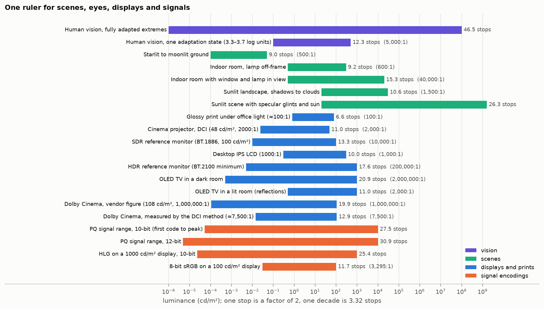
Figure 7. Scenes, vision, displays and signal encodings on a single luminance axis. Display entries are quantity A; encodings are quantity C.

6.1 Encodings (quantities C and D)

Encoding	First code to peak (C)	Span with step ≤ 5% (D)	Span with step ≤ 2% (D)
8-bit linear	8.0	3.7	2.4
8-bit sRGB	11.7	5.9	2.8
8-bit pure γ 2.2	17.6	5.5	2.6
10-bit γ 2.4, narrow range	23.5	10.0	6.9
10-bit HLG, 1000 cd/m²	25.4	11.9	8.8
10-bit PQ	27.5	17.1	12.5
12-bit PQ	30.9	21.8	18.9
12-bit linear (raw)	12.0	7.7	6.4
14-bit linear (raw)	14.0	9.7	8.4
16-bit linear	16.0	11.7	10.4

All values in stops, computed for this article [Code].

Reading the table:

• Column C is close to meaningless for a power-law curve: the pure 2.2 curve “has” 17.6 stops in 8 bits only because its lowest code is absurdly dark and its lowest steps are 100% jumps.
• Column D is what matters for banding . An honest one-line statement is “10-bit PQ gives about 17 stops with steps under 5%”.
• A linear integer with $N$ bits spans exactly $N$ stops by C, and the top stop uses half the codes (Figure 8, right).

6.2 Sensors (quantity B)

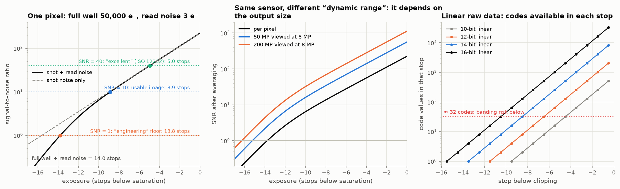
Figure 8. Left: signal-to-noise ratio of one pixel against exposure. The same pixel has 13.8, 8.9 or 5.0 stops of dynamic range depending on the SNR called the floor. Middle: averaging pixels raises SNR, so the figure also depends on the size at which the image is judged. Right: codes available in each stop of linear raw data. [calc]

• Engineering dynamic range is full-well capacity over read noise. ISO 15739 places the floor at SNR = 1, according to Imatest’s documentation [web]. ARRI’s white paper uses the same floor and cites ISO 15739 and EMVA 1288 for the general definition, saturation over sensitivity threshold [p. 7]. Imatest notes that its own procedure “differs in several details from ISO 15739”. An image at SNR = 1 is not usable; it is the point where signal equals noise.
• Photographic dynamic range (Photons to Photos) uses SNR = 20 at a normalized print size; its own example gives 9.0 against 12.4 stops, a 3.4-stop gap for the same sensor [2nd].
• Cinema camera claims use no agreed threshold. One test house maps a manufacturer’s 14-stop claim to SNR = 2 and measured about 12 on a camera claimed at 15 [2nd]. Treat claimed stops as comparable only within one source. ARRI is the one maker found that documents its method: step exposures from black to saturation, signal linearized from LogC, floor at SNR = 1, giving 17 stops for the ALEXA 35 and 14.5 for the ALEXA Mini LF. The same paper says a floor of SNR = 2 gives “at least one stop lower”, that the camera’s texture settings move the figure by −¼ to +½ stop, and that counting the last visible patch on a step chart overestimates [ARRI 2022, pp. 7–12]. Independent chart tests of the ALEXA 35 report about 15.1 stops at SNR = 2 and 16.3 at SNR = 1; a Sony camera marketed at 16 stops measured 13.0 and 14.3; RED’s “17+” appears to be a clipping-to-black range with no noise criterion [search snippets only]. Sony’s brochure for one cinema camera states exposure latitude “from 6 stops over to 10 stops under 18% Middle Gray, for a total of 16 stops”, with no noise criterion [std, Sony brochure, p. 11]; no RED document defining its figure was found. The machine-vision standard EMVA 1288 defines dynamic range as saturation over the sensitivity threshold at SNR = 1, the same floor as ARRI’s [std, EMVA 1288 release 4.0, pp. 11–12].
• Output size. Averaging $n$ pixels raises SNR by $\sqrt n$, about half a stop of dynamic range per halving of linear resolution. Scores normalized to 8 megapixels are not comparable with per-pixel figures.
• Bits are not stops. A linear ADC of $N$ bits cannot record much more than $N$ stops, but it can easily record fewer: a sensor with 11 stops of engineering range behind a 14-bit ADC has 11. In the other direction, when read noise is below one code the noise dithers the quantizer and the engineering figure can exceed $N$ by a stop or so. Sensors that claim more stops than their raw bit depth do it with dual gain readout, multiple exposures, or a companded (piecewise or log) raw encoding.

6.3 Log encodings (quantity E)

Curve	Code value of 18% gray	Stops above 18% gray at code 1.0
S-Log3	0.411	7.7
ARRI LogC3 (EI 800)	0.391	8.3
ACEScct	0.414	10.3
ARRI LogC4	—	11.4 (469.8 at hardware maximum, per the ARRI specification)

Computed from the published formulas [calc]; LogC4 from the specification [std]. These are the limits of the code range, not of any sensor.

Log curves allot a roughly constant number of codes per stop above the toe, so “stops” maps cleanly onto code range. What the curve can hold says nothing about what the sensor delivers.

6.4 Film, displays and eyes

• Film negative. Film figures are exposure latitude read from the characteristic curve, not a noise-based dynamic range. Kodak’s brochure for VISION3 500T puts a white card 2⅓ stops above an 18% gray card with “at least 3½ stops above that”, and a 3% black card 2⅔ stops below with “at least 2½ stops of latitude below that”: at least 11 stops in all [std, Kodak brochure, p. 2; the sum is computed here]. An older definition, the exposure range that produces a density change, gives “approximately ten camera stops” for a typical negative stock (Kennel and Snider 1993, p. 2). The commonly repeated “13 to 14 stops” has no source that could be found.
• Displays. Contrast is a property of the display in a room. An OLED with an unmeasurably low native black shows about 2000:1 (11 stops) once screen reflections add half a nit. A cinema figure of 1,000,000:1 is a vendor sequential-contrast number; the same system measured by the DCI method is about 7,500:1, or 12.9 stops [2nd]. The BT.2100 reference display (at least 1000 cd/m², at most 0.005) is 17.6 stops [std].
• Vision. Across full adaptation, from starlight to sunlit snow, the eye covers about 14 decades (46 stops). In a single adaptation state the simultaneous range is far smaller: 3.7 log units (12.3 stops) reported by Kunkel and Reinhard (2010) from experiments on an HDR display, under specific conditions of stimulus duration, contrast and background; and a maximum of about 3.3 log units (11 stops) measured directly by Jiang and Fairchild (2021), who say the 3.7 “was not measured directly” and that their value depends on the luminance and size of the bright stimulus. Earlier estimates span 2 to 4 log units [abstracts only]. Local adaptation while scanning a scene extends this. Numbers such as “the eye sees 20 stops” or “24 stops” mix the two.

Recommendation. Never write a bare stop count. Write the quantity and its criterion: “13.8 stops, SNR = 1, per pixel”; “17 stops with steps under 5%”; “12.9 stops, DCI method, in the auditorium”.

---

7. Bits: where the codes go, and what fits in what

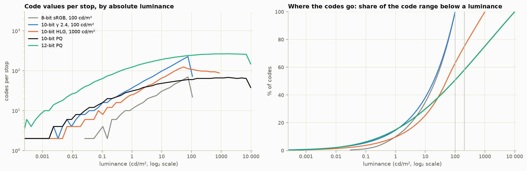
Figure 9. Left: code values per stop against absolute luminance. Right: share of the code range lying below a given luminance. [calc]

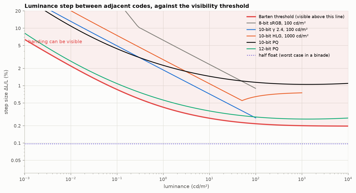
Figure 10. Relative luminance step between adjacent codes, against a Barten-model visibility threshold. The threshold is an implementation of the model with the parameters and criterion of ITU-R BT.2246 (step = 2/(1.27 S), checked against BT.2246-8, PDF p. 44, printed p. 42; the code uses a 40° field where the report uses 60°, which changes the curve by under 3%). It sits about 1.4 times lower than the curve drawn in BT.2390, which 12-bit PQ just clears. BT.2390 says only that its curve is “based on the detailed Barten model” and prints no parameters, so the gap cannot be traced to a specific choice. Ratios between encodings are unaffected. [calc]

What the two figures say:

• Gamma curves waste codes in HDR. A power law gives a constant number of codes per stop only in the sense that the number keeps falling toward black. Stretched to 10,000 cd/m², a 12-bit gamma curve is substantially above threshold in the shadows [std, BT.2390].
• 12-bit PQ is below threshold across its range. 10-bit PQ is above it, by a factor of roughly 4 at worst by this calculation, as is 10-bit BT.1886 at 100 cd/m². BT.2390 says both exceed the threshold “to some extent” and adds that realistic camera noise masks the result [std]. Noise-free content (graphics, gradients, CGI skies, denoised video) is where 10-bit banding shows. A sweep of the BT.2020 color cube (§7.5 ) puts adjacent 10-bit PQ codes about 1.2 ΔE_ITP apart at every peak, just over one just-noticeable difference [calc]; Miller’s flat-field tests needed 11 bits [2nd]. Independent support: threshold tests of HDR pixel encodings found 0.005 to 10,000 cd/m² encodable without perceptual loss in 11 bits or more, with PQ the most uniform (Mantiuk, Boitard and François 2014 [pp. 2 and 5]); a banding study found the contrast threshold highest near 0.1 cd/m² and roughly constant above 100 (Kim, Azimi and Mantiuk 2020 [abstract]); and Dolby’s own paper says “12bit PQ is below the visible threshold for contouring artefacts whereas 10bit PQ is above”, recommending 12 bits for noise-free content and calling 10 “adequate” for captured content [Dolby 2014, pp. 6–7]. The same paper puts the visibility threshold at about 2.5 ΔE2000 for noise-free content and about 5 with noise. BT.2246 reaches a similar split for gamma coding: 10 bits suffice by one criterion, and by the Barten criterion for flat patches “even 12 bits is not sufficient for some ranges of luminance”; for ramps, which it considers more representative of natural scenes, the same page concludes that “12 bits is sufficient to cause no tone jump artefact” [std, PDF p. 45].
• HLG at 10 bits is coarser than PQ in the shadows and finer in the upper midtones.
• 8 bits is not enough for PQ or HLG. Steps are over 4% everywhere.
• Half float has a constant 0.05–0.1% step: about four times finer than the threshold at any level, at 16 bits.

7.1 Packing problems

Container	What it is	What goes wrong
8-bit PQ or HLG	HDR in an 8-bit codec	Visible banding in any smooth area; needs dither at minimum
10-bit in 16-bit words (P010, P016)	Value in the high bits	Reading as a plain 16-bit integer is right; reading the low 10 bits gives noise. The opposite convention (value in the low bits, as in most yuv420p10 files) is 64× darker when misread
RGB10_A2 / A2R10G10B10	10-bit color, 2-bit alpha	Alpha has four levels; premultiplied soft edges band. Channel order differs between APIs
R11G11B10F	Unsigned small floats: 5-bit exponent (bias 15), 6-bit mantissa for R and G, 5-bit for B [std, Khronos Data Format Specification 1.3, ch. 10]	No negative values (wide-gamut colors expressed in a smaller space clip); 1.6% and 3.1% steps, so blue-yellow banding in bright gradients (Figure 11)
RGB9E5	Three 9-bit mantissas, one shared 5-bit exponent	Precision is set by the largest channel; a dim channel beside a bright one loses bits. Saturated dark colors suffer
Radiance RGBE	8-bit mantissas, shared 8-bit exponent	Same shared-exponent flaw at 8 bits; common reference code has a dark bias and twice the necessary error [prior]
Narrow range in 10 bits	64–940 (luma), 64–960 (chroma)	876 usable codes, not 1024. Codes 0–3 and 1020–1023 are reserved in SDI. Scaling 8-bit to 10-bit is ×4, not ×1023/255. That holds for narrow range only; full-range data needs the exact scale (§7.4 )
12-bit content in 10-bit streams	e.g. dual-layer or reshaped HDR	The extra precision exists only after the decoder applies metadata; a plain decoder sees 10 bits
Float 1.0 conventions	§5.4	Factor of 80 or 203 errors

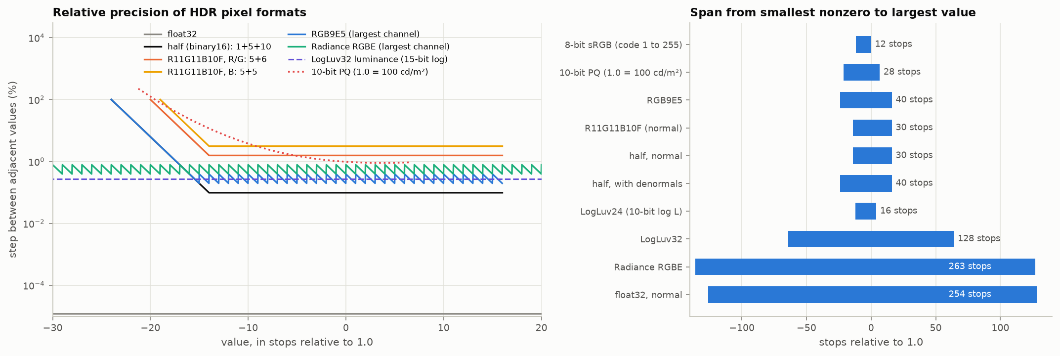
Figure 11. Left: relative step of common HDR pixel formats against value. Right: span from the smallest nonzero to the largest value. [calc]

7.2 Round trips

• Linear storage needs $n+4$ bits to hold $n$-bit sRGB without loss; 8-bit linear keeps only 183 of 256 sRGB codes [calc].
• Half float carries 8-bit and 10-bit sRGB through a decode to linear and back without loss, but loses 86 of the 4096 codes at 12 bits [prior]. Whether an 8-bit value survives a trip through a half float also depends on the rounding rule used (§7.4 ).
• Every conversion between narrow and full range, or between $Y'C_bC_r$ and $R'G'B'$ at the same bit depth, loses codes: only about one in six 8-bit RGB colors survives a trip through 8-bit narrow-range $Y'C_bC_r$ (from the count of code triples that decode to valid RGB; approximate).

7.3 Banding and dither

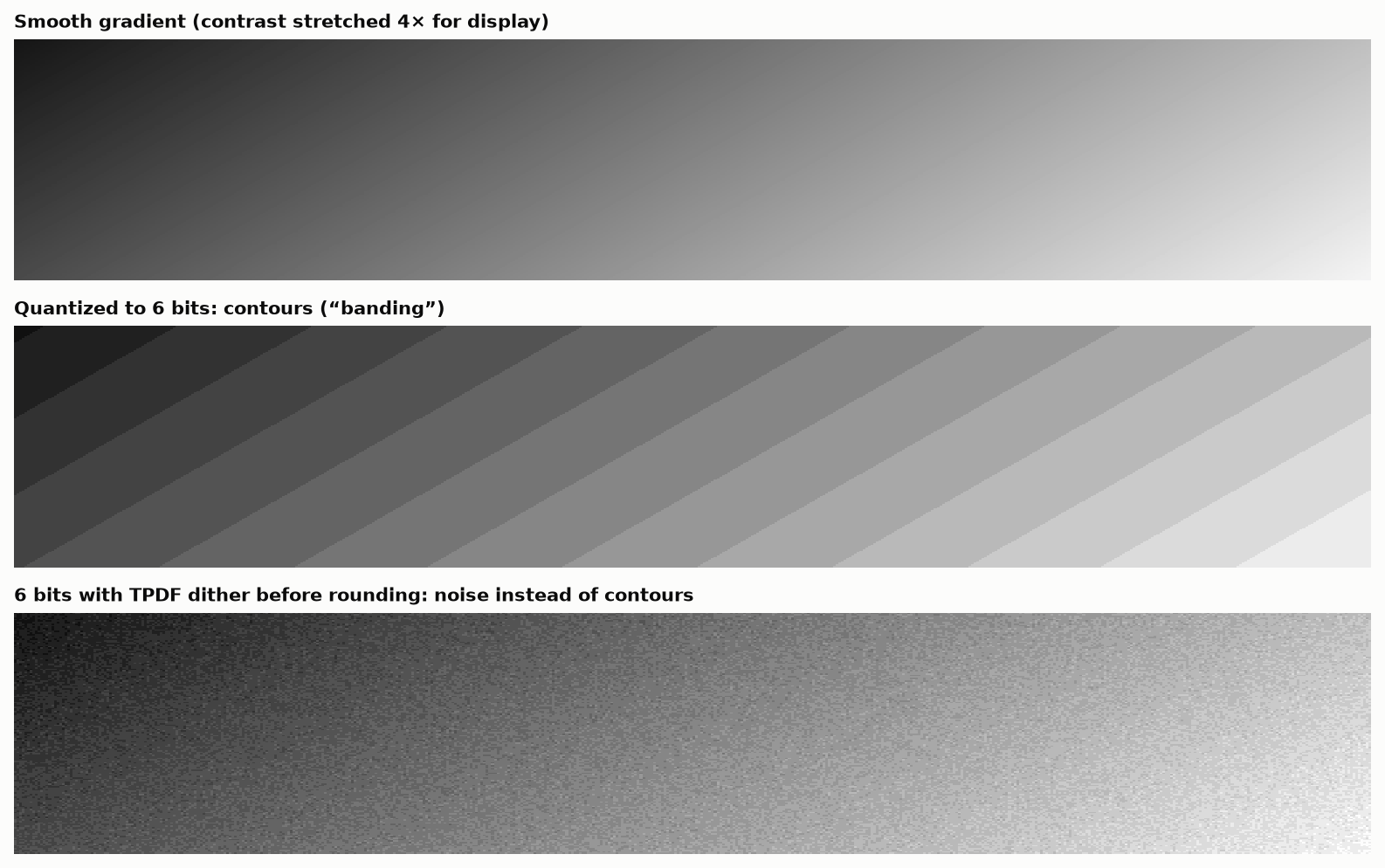
Figure 12. A slow dark gradient, quantized to 6 bits so the effect survives reproduction, without and with triangular dither before rounding.

Dither converts contours into noise whose average is the true value. It costs nothing in bit rate terms for uncompressed data and is the correct final step of any reduction in bit depth. Lossy codecs tend to remove it, which is why film grain synthesis and debanding filters exist at the decoder.

7.4 Rounding rules: bytes, floats and bit-depth changes

Most pipelines convert between floats and integer codes many times, and the conversion is usually written without thought. The results below are from exhaustive tests and short proofs. Those marked [calc] were recomputed for this article; those marked [prior] were not.

Float to byte and back. Two rules are in common use for encoding a float $f\in[0,1]$: round(255 f), which graphics hardware uses for normalized integers, and floor(256 f) clamped to 255. Two rules are in use for decoding: i/255 and (i + 0.5)/256. Only two of the four pairings are consistent.

Encode	Decode	Mean squared error (1 = best possible)	Notes
round(255 f)	i/255	1.008	The hardware rule. Exact at 0 and 1
floor(256 f)	(i + 0.5)/256	1.000	Equal-width bins. Cannot represent 0 or 1 exactly
floor(256 f)	i/255	2.008	The common mismatch. Costs half a bit at every bit depth
truncation, floor(255 f)	i/255	about 4	Costs a full bit

[calc]

The mismatched pair in the third row is worth recognizing, because it is everywhere.

• It disagrees with the hardware rule on 24.9% of inputs, by one code.
• It is the correct quantizer followed by a 0.4% contrast stretch about mid-gray: values near black come back half a code too dark and values near white half a code too bright.
• Over generations it drifts. A gray of 0.30 run through the mismatched pair with fresh dither each pass reads about 0.26 after 50 passes, 0.20 after 100, 0.06 after 200 and 0 after 300. The matched pairs stay where they are [calc].

The rule: the half step must appear exactly once, in the encoder or in the decoder, and the scale must be the same in both. Use round(255 f) with i/255 unless there is a reason not to.

Through a half float. An 8-bit value decoded with i/255 survives storage in a 16-bit float, or in a 16-bit “brain float”, and re-encodes to the same code for all 256 codes. Decoded with the mismatched rule it comes back one code high on 15 codes in a half float and on 127 in the brain-float format [prior].

Infinity and NaN. Converting an out-of-range float to an integer is undefined in C and C++. The same source code turns +∞ into black on x86 and white on ARM. Clamp in floating point first, and write the clamp so that NaN fails the comparison: if (!(x > 0)) return 0; if (x >= 1) return 255; [prior, measured].

Bit-exact tests fail for a boring reason. In 32-bit float, (int)(x*255.0f + 0.5f) and nearbyint(x*255.0f) each misround 128 of the roughly one billion floats in [0, 1], because the product is rounded before the add. Form the product in double precision, where it is exact [prior, exhaustive].

Changing bit depth. Shifting is exact only for narrow range, where the standards define the levels as multiples (16 becomes 64, 235 becomes 940). For full range:

Operation	Shortcut	What goes wrong	Exact form
8 to 10 bits	v << 2	White becomes 1020; 213 of 256 codes wrong, by up to 3	round(v * 1023 / 255)
10 to 12 bits	v << 2	White becomes 4092	round(v * 4095 / 1023)
16 to 8 bits	v >> 8	Wrong on 24.8% of values	(v * 255 + 32895) >> 16
5 to 8 bits	v << 3	White becomes 248	replicate the top bits into the bottom

[calc]

Multiplying two 8-bit values (alpha blending, premultiplying). (a*b) >> 8 is wrong for 72% of the 65,536 input pairs and (a*b)/255 with truncation for 48%. Exact forms, all verified exhaustively: with t = a*b + 128, (t + (t >> 8)) >> 8; or (t * 257) >> 16; or (2*a*b + 255) / 510 [calc].

Premultiplied alpha in 8 bits is lossy. A channel stored as color times alpha has only alpha + 1 distinct levels, so at an alpha of 8/255 a channel has nine. Premultiplying, storing in 8 bits and dividing again returns the original for only half of all color and alpha pairs. And premultiplying encoded values, which many image loaders do, is the Section 10 error again: an sRGB white at half coverage is stored as code 127, which is 21% of the light instead of 50% [prior].

How many linear bits hold an encoded image? Decoding 8-bit sRGB to linear integers and re-encoding loses 73 codes if the linear values have 8 bits, 39 at 9, 18 at 10, 6 at 11 and none at 12. The same pattern holds at 10 bits (none lost at 14). So exact round trips need four more linear bits than encoded bits [calc]. Other criteria give other numbers: 13 bits to match the first sRGB step, 17 to match every step of a gamma-2 curve. When someone quotes a required linear bit depth, ask which criterion.

Black subtraction and clipping. Clamping zero-mean noise at zero adds a bias of $\sigma/\sqrt{2\pi}$, about 0.4σ. In raw processing that lifts the shadows, and tints them when the noise differs by channel [calc].

7.5 HDR bit depth, measured one way

A direct measurement complements the threshold curves of Figure 10. Quantize each channel of BT.2020 RGB uniformly in the encoded domain, sweep the color cube up to a given peak, and record the largest $\Delta E_{ITP}$ produced by moving one channel by half a code (the worst rounding error) and by a whole code (the step between neighboring colors). A value of 1 is about one just-noticeable difference under the most critical conditions.

Encoding	Rounding error, 100 cd/m² peak	1000 cd/m²	10,000 cd/m²	Step between adjacent codes at 10,000 cd/m²
PQ, 8-bit	2.3	2.3	2.4	4.9
PQ, 10-bit	0.57	0.58	0.61	1.2
PQ, 11-bit	0.28	0.29	0.30	0.61
PQ, 12-bit	0.14	0.14	0.15	0.30
Linear, 16-bit integer	4.7	16	48	64
Linear, 20-bit integer	0.92	3.6	13	18
Linear, 24-bit integer	0.18	0.70	2.7	4.1

[calc] Worst case over the cube, no noise, one channel moved at a time.

Three things follow.

• Each added bit halves the error, for every encoding.
• PQ’s error barely depends on the peak. That is what the curve was designed for. Ten-bit PQ rounds to within 0.6 of a just-noticeable difference, but neighboring codes are 1.2 apart, which is why clean gradients can show steps at 10 bits and not at 12.
• Linear integers need about 26 bits to match 10-bit PQ’s rounding error at a 10,000 cd/m² peak, and 22 at 100 cd/m². The worst case is always near black, where a linear step is a large fraction of the value.

The numbers compare encodings fairly and should not be read as absolute visibility thresholds: the criterion is a worst case that real content rarely presents.

---

8. A color float: design study

The ingredients are simple: an unsigned float with an exponent bias and no sign bit; a normalized mantissa with an implied leading one; and, as the smallest useful case, a 4-bit exponent with a 12-bit mantissa in 16 bits. A related measurement points the same way: linear luminance plus two chroma channels at 14, 13 and 13 bits beats 10-bit PQ, while 32 and 36 bits in total do not [prior]. The analysis below uses luminance steps against the Barten threshold only. It should be repeated with $\Delta E_{ITP}$ over the full color cube before any conclusion is treated as final.

8.1 What color needs from a float

IEEE half float was designed for general arithmetic. For display-referred color it spends bits badly:

Half-float feature	Use for color
Sign bit	None for luminance. Needed only for out-of-gamut values in a smaller RGB space
30 normal binades, 2⁻¹⁴ to 2¹⁵	Display light needs about 21 (0.005 to 10,000 cd/m²); scene light perhaps 30
Infinities and NaNs (a full exponent code)	Harmful; saturation is the right overflow behavior
Same mantissa width in every binade	The eye tolerates 6% steps at 0.001 cd/m² and needs 0.2% at 1000

BFloat16 answers a different question (keep float32’s range, drop mantissa to 7 bits) and has 0.4–0.8% steps: too coarse for color at 16 bits.

8.2 Uniform-mantissa unsigned floats, exmy

Take $e$ exponent bits and $m$ mantissa bits, no sign, hidden leading one, exponent code 0 for a denormal binade, and scale so the largest value is 10,000 cd/m².

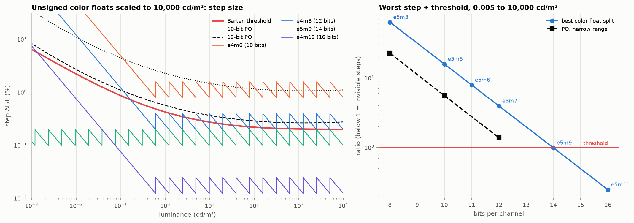
Figure 13. Left: step size of four layouts against the threshold and against PQ. Right: worst step divided by threshold over 0.005 to 10,000 cd/m², for the best split at each width. [calc]

Bits	Best split	Worst step ÷ threshold	Smallest nonzero (cd/m²)	Mantissa step	Comparable PQ
8	e5m3	63	6×10⁻⁷	12.5%	8-bit PQ: 23
10	e5m5	16	1.5×10⁻⁷	3.1%	10-bit PQ: 5.6
11	e5m6	7.9	7×10⁻⁸	1.6%
12	e5m7	3.9	4×10⁻⁸	0.78%	12-bit PQ: 1.4
14	e5m9	0.99	9×10⁻⁹	0.20%
16	e4m12	0.49	7×10⁻⁵	0.024%
16	e5m11	0.25	2×10⁻⁹	0.049%

Findings [calc]:

• A uniform-mantissa linear float costs about two bits more than PQ for the same worst-case visibility: e5m7 (12 bits) is a little better than 10-bit PQ, and e5m9 (14 bits) a little better than 12-bit PQ. An earlier estimate by a different route agrees.
• Four exponent bits are not quite enough for the full range at small widths. e4 has 15 normal binades: with the top at 10,000 cd/m² the normal range ends at 0.3 cd/m², and everything darker is in the denormal binade with a fixed absolute step. At 16 bits (e4m12) the denormal step is small enough that it stays under threshold down to 0.005 cd/m². At 12 bits (e4m8) it does not.
• Five exponent bits waste range. 31 binades reach 10⁻⁸ cd/m², ten binades below anything a display or the eye needs.
• The implied leading one matters: without it the representation is redundant and the top bit of the mantissa is wasted in every binade but the lowest.

8.3 Two improvements specific to color

(a) A non-power-of-two exponent count. Nothing forces the number of binades to be 16 or 32. Give the format $B$ binades and $M$ steps per binade, with code $= B_{\text{index}}\cdot M + \text{step}$. Decoding is one integer divide (or a small table) and one shift. With $B = 21$ binades covering 0.005 to 10,000 cd/m², a 12-bit word has $M = 195$ steps per binade (0.51%) against 128 (0.78%) for e5m7.

(b) A tapered mantissa. Let the number of steps per binade follow the visibility threshold: few in the dark, many in the bright. The decoder needs a 21-entry table of (first code, step size). For steps exactly at threshold over 0.005 to 10,000 cd/m² [calc]:

Design	Codes needed	Bits
Ideal curve (every step at threshold; this is what PQ approximates)	4,542	12.15
Tapered float: linear within each binade, steps per binade from 33 (darkest) to 505 (brightest)	6,327	12.63
Uniform-mantissa float, 21 binades	10,605	13.37

So a tapered linear float sits about half a bit above the perceptual optimum and three-quarters of a bit below a uniform float. The half bit is the price of being piecewise linear: within a binade the relative step varies by a factor of two.

What that half bit buys is the property PQ lacks: the value is linear light within each segment, decoding needs no power functions, and blending or filtering two values in the same binade is exact integer arithmetic. Whether that is worth it depends on the use. For storage and transport PQ is already near-optimal. For a working format on a GPU without fast transcendental functions, or for textures that are filtered in hardware, a tapered float is a credible design.

8.4 Candidate layouts

Name	Layout	Range (1.0 = 203 cd/m²)	Notes
cf16	e4m12, unsigned, saturating	7×10⁻⁵ to 10,000 cd/m²	The plain layout. Below threshold everywhere; four times finer than half float in its normal range
cf14	e5m9, or 21 binades × 780 steps	to 10,000 cd/m²	At threshold. Three channels fit in 42 bits; with 2 spare bits per 16-bit word
cf12-t	tapered, 21 binades, table-driven	0.005 to 10,000 cd/m²	About 1.5× threshold at 4,096 codes: between 10-bit and 12-bit PQ in quality, linear within segments
cf10-t	tapered	same	About 6× threshold: no better than 10-bit PQ. Not recommended
cf32 RGB	Shared exponent done properly: 5-bit exponent + 3 × 9-bit mantissa (this is RGB9E5)		Already exists; the weakness is saturated darks
cf32 YCC	14-bit tapered $Y$ + 2 × 9-bit chroma ratios		Combines the float with a linear luma and chroma split; chroma needs testing, since chroma error dominates at 9 bits or fewer

Open questions: (1) rerun the table with ΔE_ITP over the BT.2020 cube rather than luminance alone; (2) decide whether 1.0 is 203 cd/m² or peak; (3) measure the cost of hardware bilinear filtering across a binade boundary in the tapered format; (4) compare with the IEEE P3109 draft, which defines small saturating unsigned floats for machine learning and is the nearest existing template.

---

9. Luma, chroma and subsampling

9.1 What $Y'C_bC_r$ is

$$Y' = K_R R' + K_G G' + K_B B',\qquad C_b = \frac{B'-Y'}{2(1-K_B)},\qquad C_r = \frac{R'-Y'}{2(1-K_R)}$$

computed from encoded $R'G'B'$. The coefficients come from the luminance row of the RGB-to-XYZ matrix for the primaries in use:

Standard	$K_R$	$K_G$	$K_B$
BT.601	0.299	0.587	0.114
BT.709	0.2126	0.7152	0.0722
BT.2020	0.2627	0.6780	0.0593

“YUV” is the analog PAL name and is used loosely for all of these. $Y'$ is luma, not luminance: because it is a weighted sum of encoded values, part of the true luminance ends up in the chroma channels (non-constant luminance). Three other forms exist: BT.2020 constant-luminance $Y'_C C'_{bc} C'_{rc}$ (rarely used), ICtCp (PQ- or HLG-encoded LMS, designed for HDR, much better hue linearity and luminance separation), and reversible integer transforms such as YCgCo.

9.2 The J:a:b notation

Notation	Chroma resolution	Typical use
4:4:4	full	RGB, graphics, mastering
4:2:2	half horizontal	production video, SDI
4:2:0	half horizontal, half vertical	nearly all distribution video, JPEG photos, HEIC
4:1:1	quarter horizontal	DV (NTSC)
4:0:0	none	monochrome
4:4:4:4	full, plus alpha	compositing

Chroma siting (where the chroma sample sits relative to the luma samples) differs: centered between samples in JPEG and MPEG-1, co-sited with the left column in MPEG-2 and H.264, co-sited top-left for BT.2020 UHD. Getting it wrong shifts color by half a pixel: fringes on one side of every colored edge.

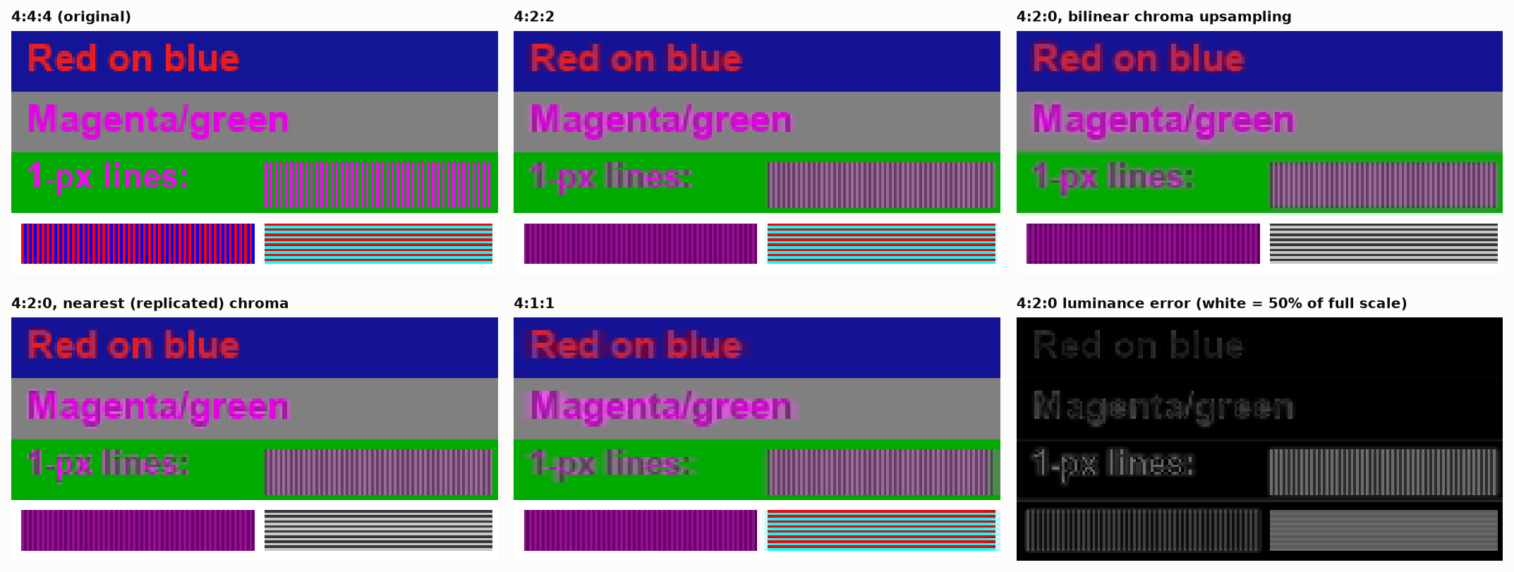
Figure 14. A test pattern through chroma subsampling. Text edges smear; one-pixel red and blue lines lose more than half their luminance. Bottom right: luminance error for 4:2:0. [calc]

The luminance loss is the important and less-known failure. Averaging the chroma of adjacent red and blue pixels and reconstructing gives purple pixels whose luminance is too low: in the figure the line pattern drops from a mean luminance of 0.142 to 0.064 [calc]. This is non-constant-luminance leakage. It is worse with PQ, whose steeper curve makes $Y'$ a poorer proxy for luminance, and it is why HDR10 encoders adjust luma after chroma downsampling and why ICtCp exists.

How large the errors are. Chroma operations on a non-constant-luminance signal change luminance, and with PQ the effect is large [calc]:

• A pure BT.2020 blue at 100 cd/m² has a luminance of 5.9 cd/m². Halve its $C_b$ and $C_r$, as a crude subsampling filter next to a neutral pixel would, and it decodes to 0.40 cd/m², fifteen times darker. Zero the chroma and it is 0.02.
• A pure red at the same level goes from 26.3 to 3.5 cd/m².
• A saturated sRGB red and a gray with the same luma differ in luminance by a factor of 5.7.

Other numbers worth having: only about a quarter of the $Y'C_bC_r$ code cube corresponds to valid RGB, so roughly two bits in thirty carry nothing [prior, computed]. Using BT.601 weights where BT.2020 is meant shifts luminance by 4% of full scale for red, 9% for green and 6% for blue. A skin tone moves 7 or 8 codes in chroma between the BT.601 full-range and BT.709 narrow-range forms, so fixed chroma-key and skin-detection thresholds silently depend on matrix and range [prior, computed]. And the ICtCp matrix for HLG is not the PQ one: its $C_t$ row is 0.548 times the PQ row and its $C_p$ row 0.530 times, so applying the PQ matrix to an HLG signal makes $C_t$ about 1.82 times and $C_p$ about 1.89 times too large [std; calc].

---

10. Arithmetic in the right space

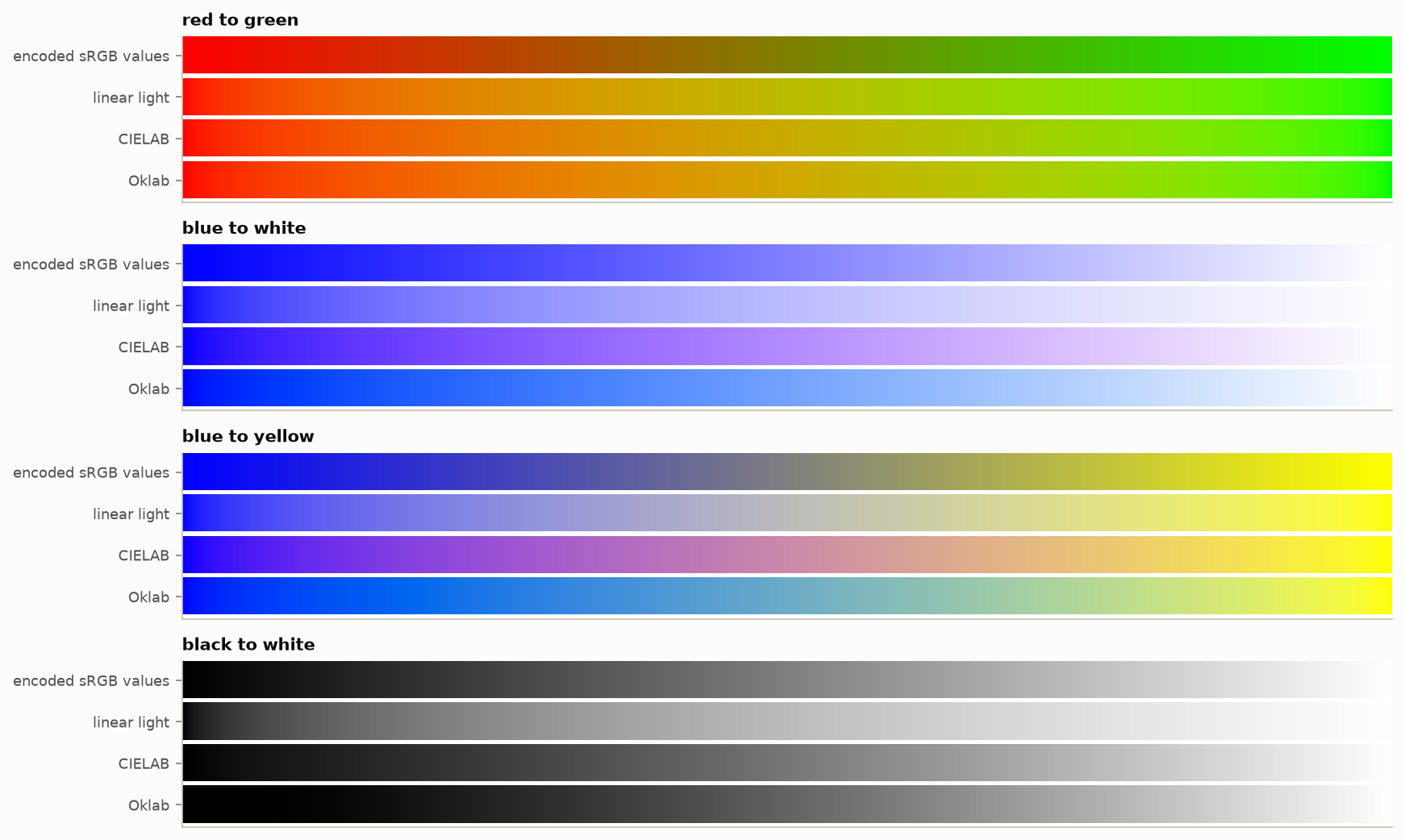
Figure 15. The same four gradients interpolated in four spaces. Encoded sRGB darkens the middle of red-to-green. CIELAB turns blue-to-white purple. Linear light is physically right and perceptually uneven. Oklab is even and keeps hue.

• Physical operations in linear light: blending, antialiasing, resizing, blur, lighting, adding gain maps. Doing these on encoded values darkens mixtures of saturated colors; the worst-case error is about 0.29 of full scale [calc].
• Perceptual operations in a perceptual space: gradients meant to look even, gamut mapping, color-difference measurement, dither and quantization decisions, sharpening (the Hoppe distinction covered in the Image Processing notes).
• Pick the perceptual space with care. CIELAB has a known blue hue nonlinearity. Oklab fixes it for SDR. ICtCp and $J_za_zb_z$ were built for HDR. None includes the H–K effect.

10.1 Tone mapping and the hue of highlights

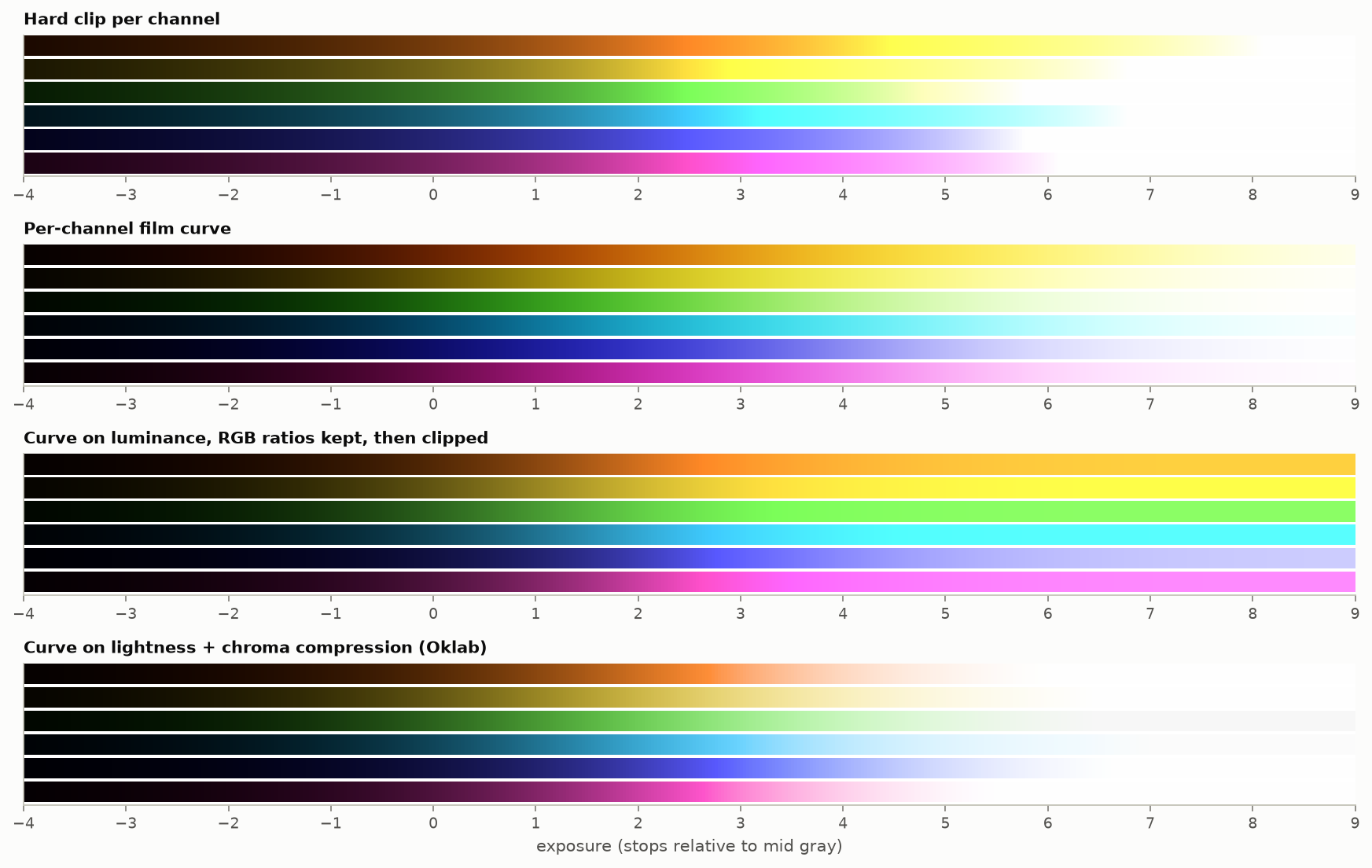
Figure 16. Six saturated colors swept through 13 stops of exposure under four highlight strategies. [calc]

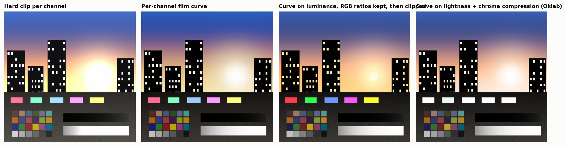
Figure 17. The same four strategies on a synthetic HDR scene with a sun, saturated signs brighter than white, and deep shadows.

• Hard clip per channel: as one channel saturates, the ratios change. Orange turns yellow, blue-cyan turns cyan, then everything turns white. Seen as yellow rings around the sun and cyan skies.
• Per-channel curve: smooth, film-like desaturation toward white, with the same hue skews in gentler form (red toward orange and yellow, blue toward cyan). Most “filmic” operators and many camera pipelines behave this way.
• Curve on luminance, ratios preserved: hue is exact while the color stays in gamut, but bright saturated colors cannot be reached by the display and clip flat: no highlight roll-off, neon-looking lights.
• Curve on lightness plus chroma compression in a perceptual space: closest to the intent; needs a gamut-mapping step and a choice of space, and is where current work (ACES 2.0, BT.2390 and BT.2446 methods, vendor mappers) differs.

No strategy preserves hue, saturation and brightness at once. The display’s color volume is smaller than the scene’s, and something must give.

10.2 Gamut mapping

Converting BT.2020 to BT.709 with a 3×3 matrix yields negative and over-range values for out-of-gamut colors. Clipping them changes hue; compressing toward gray changes in-gamut colors too. ITU-R’s own report on the subject concluded that its requirements cannot all be met at once (“no universal gamut mapping method … can achieve all of these requirements simultaneously”) and that only methods that clip to the gamut boundary (matrix-and-clip, and a boundary mapping in CIELAB) leave in-gamut colors alone and survive repeated round trips, while compressive methods are invertible but alter in-gamut colors [prior, from BT.2407].

The hue shift from clipping depends on brightness. Converting BT.2020 to BT.709 by the exact matrix and then clipping each channel shifts the CIELAB hue of a saturated green by about −10° and cuts its chroma from 208 to 120. More troublesome, the shift changes with level: a BT.2020 orange moves +3.6° at full brightness, −3.3° at 80% and −4.7° at 50%, so an object changes hue as it dims [prior, computed]. Under a constant-hue clip in CIELAB, bright saturated yellow turns into a blown-out white patch and clipped cyan looks green; BT.2407 documents a correction that bends the mapping path for those two regions [std].

---

11. Gain maps and Ultra HDR

11.1 The mechanism

A gain-map file is an ordinary SDR image plus a second, usually smaller image holding a per-pixel log ratio between the HDR and SDR renditions. In the Ultra HDR form [std, Ultra HDR v1.1 specification]:

$$\text{HDR} = (\text{SDR}_{lin} + k_{sdr})\cdot 2^{\,G\cdot W} - k_{hdr},\qquad G = g_{min} + (g_{max}-g_{min})\,\text{map}^{1/\gamma},$$

with offsets $k$ defaulting to 1/64 and a weight $W\in[0,1]$ computed from the display’s current headroom between two metadata limits. A legacy viewer shows the SDR image; an HDR viewer boosts it by as much of the map as the screen can show at that moment. The metadata fields are Version (required), GainMapMin, GainMapMax, Gamma, OffsetSDR and OffsetHDR, each with one value or three (per channel), and the single-valued HDRCapacityMin and HDRCapacityMax; BaseRenditionIsHDR is optional and must be false. Three rules in the specification matter for the failures below: a file with invalid metadata is shown as plain SDR; the map’s own color profile and orientation tag are ignored; and a decoder that applies the map by linear interpolation instead of exponentiation gets tonal relationships that “are correct only at max content boost”.

The format: an 8-bit JPEG base, an 8-bit JPEG gain map stored after it, metadata in XMP (Google and Adobe forms) and, since ISO 21496-1 was published in July 2025, in an ISO block. The specification recommends a single-channel map at one quarter of the resolution per axis [std]. Apple’s “Adaptive HDR”, Adobe’s gain maps and Android’s Ultra HDR v1.1 specification describes how one JPEG can carry both its own and ISO 21496-1 metadata around a single gain map [std]; Apple’s documentation says its software converts ISO gain maps to headroom-adaptive metadata on decode, with a 203 cd/m² reference white, and the ICC added a tag for such gain curves in April 2025 [web].

The appeal is real: one file, backward compatible, adapts to headroom, and the author controls both renditions.

11.2 Failure modes

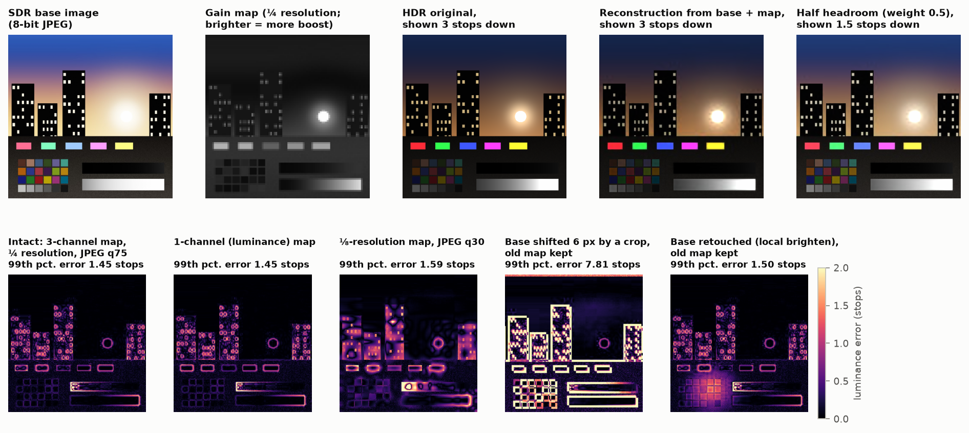
Figure 18. Top: base image, gain map, the HDR original and its reconstruction (shown three stops down so highlights are visible), and a half-headroom rendering. Bottom: luminance error of the reconstruction for five cases. Simulated with 8-bit JPEGs as in the specification. [calc]

Measured on the synthetic scene [calc]:

Case	99th-percentile luminance error	Mean error
Intact file: 3-channel map, ¼ resolution, JPEG quality 75	1.45 stops	0.16 stops
Single-channel map	1.45 stops; chroma error 3× the 3-channel case	0.16 stops
⅛-resolution map, JPEG quality 30	1.6 stops	0.25 stops
Base shifted 6 pixels by a crop, old map kept	7.8 stops	1.0 stop
Base retouched locally, old map kept	1.5 stops	0.22 stops

Evidence outside this simulation is thin. A second search found no peer-reviewed measurement of gain-map artifacts. The one technical source is a 2025 preprint that replaces the downsampled, JPEG-compressed map with a small neural network because such maps “can result in unwanted artifacts”. On 146 test images with a quarter-resolution map it reports 38.3 dB PSNR and ΔE_ITP 9.6 for a JPEG-coded map against 47.6 dB and 4.3 for its method at a smaller size, and lists “banding, haloing, block based artifacts, and loss of high frequency detail” for the conventional maps (Canham and co-authors 2025, preprint [abstract; Table 1, p. 7]). That is consistent in kind with the first rows of the table above. Reports of maps being stripped on upload (a WordPress ticket, forum threads) are anecdotes.

The failure modes, grouped:

1. Edge halos, even in an intact file. The map is low resolution and the gain changes by several stops across a sharp edge between a light source and a dark surround. The upsampled map is wrong within a few pixels of every such edge (the rings in the bottom-left panel). The gain map carried 7% of the file size here; that is the trade.
2. Desynchronization. Any edit that changes the base without regenerating the map (crop, rotate, resize, retouch, filter) leaves the two inconsistent. Android’s own documentation says complex edits leave the map unchanged unless the app handles it, and libvips warns that geometry operations leave them mismatched [2nd]. The result ranges from halos to a ghost of the original picture in the highlights.
3. Stripping. Any tool that rewrites the JPEG without understanding the appended image drops it: content management systems, image optimizers, messaging apps, some social uploads. The picture silently becomes SDR. A report of a publishing platform doing exactly this is in the notes [2nd].
4. Quantization. The base is 8-bit, already tone-mapped and lossy. The map is 8-bit over its full range, about 0.014 stop per code for a typical range [prior], then JPEG-compressed. Dark areas with large gain show amplified base-image blocking and banding. There are effectively two 8-bit images standing in for one 10- or 12-bit image.
5. Single-channel maps cannot change color. If the SDR rendition desaturated or hue-shifted the highlights (as any per-channel curve does, §10.1 ), a luminance-only gain restores brightness but not color. Saturated lights stay pale in HDR.
6. Gamut. In Ultra HDR the HDR rendition inherits the base image’s color profile [std]. An sRGB base cannot yield BT.2020 highlights.
7. Intermediate headroom. At partial weight the result is an interpolation in log space between two authored renditions, which neither was graded for. The specification warns that interpolating linearly instead of exponentially breaks tonal relationships [std].
8. Unstable appearance. Available headroom changes with screen brightness and ambient light, so the same file looks different from minute to minute and across platforms. One photographer’s tests report one browser decoding to a fixed headroom and tone-mapping while another adapts [2nd]. The CSS dynamic-range-limit property exists because a single bright HDR image in a feed was otherwise uncontrollable [2nd].
9. Metadata variants. Files in circulation carry Google-only, Adobe-plus-ISO or ISO-only metadata, and readers differ in which they accept [2nd].
10. Unspecified math space. ISO 21496-1 leaves the color space of the gain arithmetic to a flag, and implementations differ [prior].
11. Integrity. The HDR rendition can be an unrelated picture. This is demonstrable with ordinary tools, and it is the reason a gain map should be treated as content, not metadata [prior].
12. Automatic conversion of a true HDR image into base plus map is, in the words of one advocate of the format, “almost universally terrible” when left to tools [2nd].

The search found no peer-reviewed measurement of halo or banding visibility for gain maps; the evidence is specifications, bug reports and practitioner tests. That is a gap worth filling, and Figure 18’s method is a start.

11.3 Making gain maps: details that decide the result

From tests with the public reference encoder and real files [prior, measured; encoder versions not recorded]:

• Offsets. Offsets near zero stretch the 255 map codes over about 19 stops and waste them on noise in the blacks. The default of 1/64 exists for that reason. An interface that takes offsets in cd/m² needs them scaled by the reference white.
• Compute the map against the base the decoder will see. The base image is compressed, so the decoder’s base differs from the original. Computing the map from the original base roughly doubled the mean reconstruction error (0.043 against 0.023 stops) on one test image.
• Do not desaturate the SDR highlights to make them fit. That widened one channel’s gain range to 7.7 stops. Scaling out-of-range colors instead avoided it.
• Per-channel metadata. A reader that parses only single-valued attributes fails on files that store three values per field.
• Precision. One 8-bit code is 0.014 stop when the map spans 3.5 stops, 0.022 at 5.6 and 0.030 at 7.7 [calc].
• Headroom is quoted three ways. Over a 203 cd/m² white, a PQ signal has $\log_2(10000/203)=5.6$ stops and a 1000 cd/m² HLG signal 2.3, or 3.2 with super-whites. A figure of 3.6 stops for HLG takes the scene-linear value 1/12 as SDR white. Say which white is meant.
• Order of resampling. Upsampling the map in encoded form, in log form, or after converting to a linear gain gives different edges around small highlights. Encoder and decoder must agree.

---

12. Recognizing errors by their look

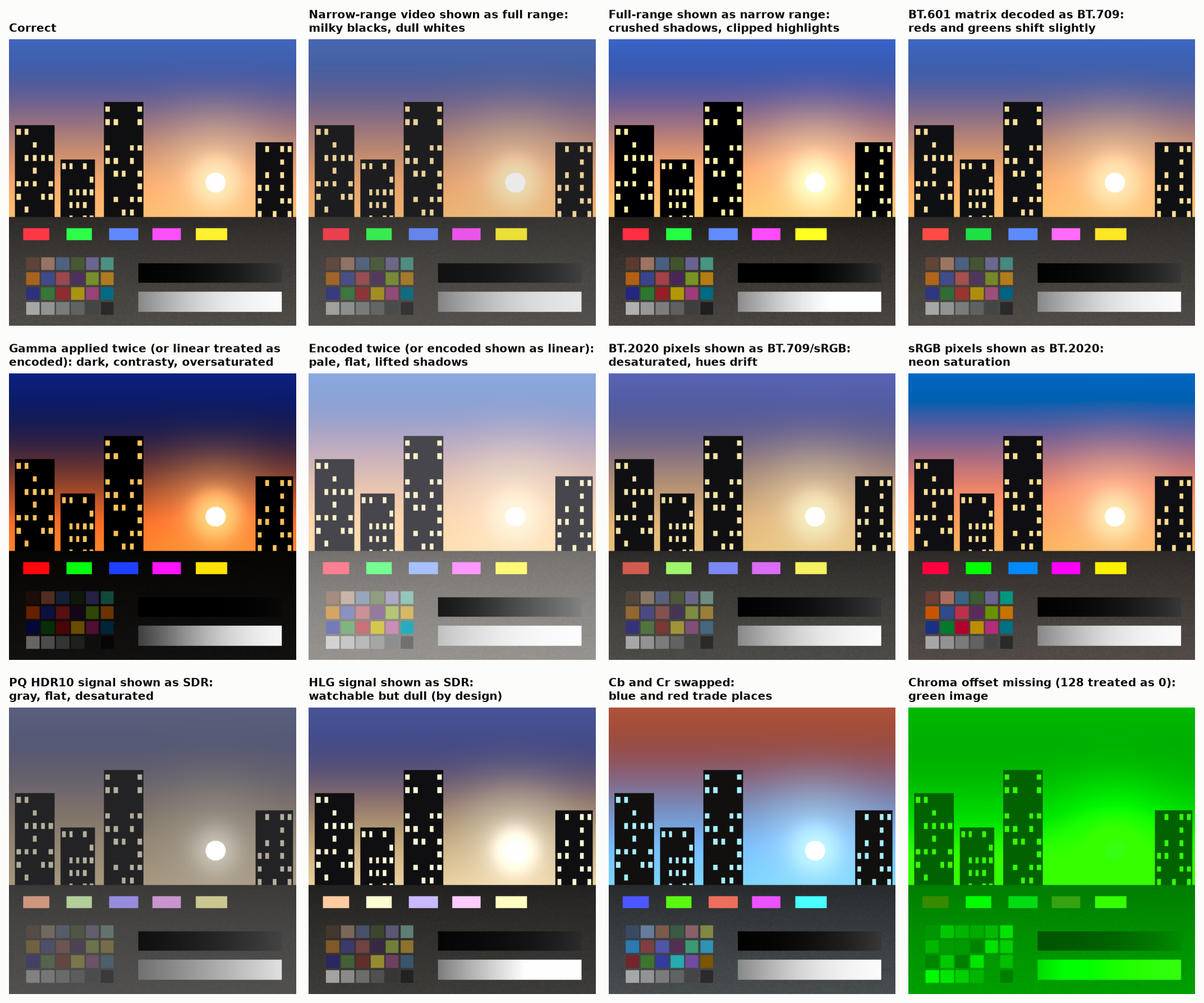
Figure 19. One correct rendering and eleven common mistakes applied to it.

The companion file Best Practices and Gotchas lists symptoms with causes and tests. The short version: washed out means a range or transfer mismatch upward; crushed means the reverse; desaturated means wide-gamut data read as narrow; neon means the opposite; green or magenta casts mean chroma offsets or plane order; a correct picture with wrong reds and greens on skin means the 601/709 matrix.

12.1 Constants and tags that circulate wrongly

Much color code is written from slides, forum posts and earlier code. These are the errors that keep being copied [prior, each checked against the standard named; computed where a number is given].

What circulates	What is right	Size of the error
sRGB thresholds 0.03928 and 0.00304 (from the 1996 proposal and the 1997 draft; still in accessibility guidelines and older code)	0.04045 and 0.0031308	At most 8×10⁻⁷ in linear light; no 8-bit code changes, 36 codes at 16 bits
BT.709 and BT.2020 curve constants 1.099 and 0.018	The values that make the curve continuous are 1.0992968 and 0.0180540; the printed ones are rounded	A step of 2.5×10⁻⁴ at the join, a quarter of a 10-bit code
The sRGB matrix inverse to four decimals	Not the inverse of the four-decimal forward matrix; white comes back as 1.000015, 1.000054, 1.000016. The standard supplies seven decimals for 16-bit work	Visible only in repeated conversions
PQ constants to four decimals, from the original paper	The exact rationals of ST 2084 (reference tables)	Code built from the rounded constants is not ST 2084
“The BT.2390 tone curve” with no edition	The Hermite roll-off moved; cite BT.2408 Annex 5, or BT.2390 with its edition	Readers cannot find it
An sRGB exponent of 2.6	2.6 is the DCI cinema exponent	Large
CIELAB constants 0.008856, 7.787, 903.3	216/24389, 841/108, 24389/27	A tiny discontinuity at the join
D65 as x = 0.3127, y = 0.3290 everywhere	The standards use those four digits; tables and formulas give 0.31271 to 0.31273 and 0.32902 to 0.32913	Matrices from different sources disagree in the fourth decimal

Tag and code-point traps in H.273 and the formats that use it:

• Range flag. The full-range flag defaults to narrow. A file tagged sRGB with the flag left at zero declares narrow-range sRGB, which is legal and almost never what the writer meant. It is a common mistake in AVIF, HEIF and PNG writers.
• No code point exists for BT.1886, Adobe RGB, ProPhoto, ACES or any D50 space. Files in those spaces need an ICC profile.
• sYCC is the BT.601 matrix on BT.709 primaries. Older files signal it with the BT.709 matrix code.
• P3 in $Y'C_bC_r$ needs the “derived from primaries” matrix codes. Using BT.709 or BT.2020 weights for P3 primaries is a matrix mismatch.
• PNG allows one ICC profile chunk, but files carry several color chunks that contradict each other, and decoders differ in which they obey. PNG alpha is always straight, never premultiplied.
• ICC version 2 and version 4 encode Lab differently in lookup tables (white is FF00 in one and FFFF in the other). Reading one with the other’s rule gives $L^{\ast}=99.6$ for white and a slight tint. ICC display calibration has no HDR model; HDR enters only through the code-point tag added in version 4.4.
• Tools report their own working space. One operating-system image tool reports two quite different raw files as the same 16-bit, three-channel, wide-gamut image, because it reports what it decoded to. Read the tags themselves.

---

13. Directions

13.1 More than three primaries

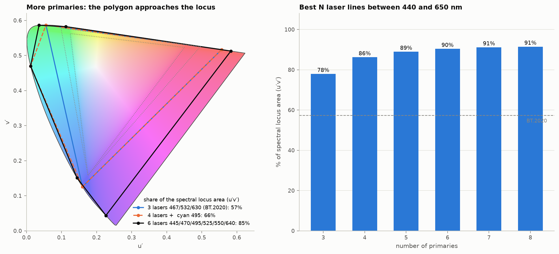
Figure 20. Left: polygons from three, four and six laser lines. Right: the best possible gamut from N laser lines between 440 and 650 nm, as a share of the spectral locus area in u′v′. [calc]

Three lasers at the BT.2020 wavelengths cover 57% of the locus. The best three lines in a practical wavelength range reach 78%, four reach 86%, six reach 90%, eight 91% [calc]. Gamut alone gives sharply diminishing returns after four or five primaries, and the remaining area is deep violet and far red, where the eye’s sensitivity is low and almost no real surface colors lie.

The stronger argument for more primaries is metamerism (§2.2 ). With $N>3$ primaries each color has an $(N-3)$-dimensional family of spectra that match for the standard observer, and the display can choose the member that matches for the most people or that is closest to a broadband spectrum. Long and Fairchild’s work at RIT modeled eight primaries and built a seven-channel projector on this basis. Long’s dissertation reports that the prototype was “proven in forced-choice paired comparison tests to deliver superior color matching to reference stimuli versus both contemporary standard RGB cinema projection and recently ratified standard laser projection”, that modeled conventional systems are worse “by a factor of 2x to 3x”, and that BT.2020 laser primaries “are likely to deliver greatly exaggerated inconsistency of experience amongst cinema audiences” [Long 2015, abstract and PDF pp. 127 and 191]. A four-primary analysis claims a large cut in observer error [2nd]. No prototype with measured observer-metamerism benefit has been published since, in what was searched. Other uses of the freedom: lower power, lower speckle , lower blue-light dose.

Corrections to common belief [2nd]:

• “6P” laser cinema projectors use two offset RGB sets, one per eye, for 3-D. They are not six-primary color systems.
• The search found no commercial display that uses more than three primaries for color. Four-color (RGBY) and RGBW panels shipped, but the fourth sub-pixel served brightness, and the signal chain stayed three-channel.
• Prototypes with five to seven primaries exist in research labs. The obstacles are the signal format (everything from cameras to codecs is three-channel), the lack of a standard way to split a tristimulus value into $N$ drives, and cost.

13.2 Other directions

• RGB backlights and micro-LED. 2025–2026 televisions with red, green and blue LED backlights measure 87–93% of BT.2020 [2nd]. Narrower primaries bring the observer problem to the living room.
• Observer-aware calibration. Individual observer models (Asano and Fairchild) and physiological models with age and field size (CIE 170-1) make per-user or per-population calibration possible. No standard carries an observer tag.
• Spectral and multispectral capture to remove camera metamerism at the source.
• Appearance-aware HDR. Models that include H–K, the Hunt effect and adaptation, used for tone mapping and for brightness specification in place of nits.
• Standards in motion (2025–2026): ISO 21496-1 (gain maps, 2025); SMPTE ST 2094-50 (headroom-adaptive tone-mapping metadata, approved August 2026) [2nd]; PNG Third Edition with cICP, mastering-display and content-light chunks (W3C Recommendation, June 2025) [2nd]; ISO TS 22028-5 for HDR stills; BT.2100-3 (2025); CSS Color HDR (working draft).
• Better pixel formats. §8 .

---

14. Known, unknown, contested

Well established

• Color matching is linear over the range of displays; XYZ arithmetic is exact for a given observer.
• The 1931 observer is wrong in the blue; cone-fundamental observers are better for narrowband light.
• 12-bit PQ is visually lossless for luminance; 10-bit is marginal on clean content; 8-bit HDR bands.
• Blending and resampling belong in linear light.
• Non-constant-luminance chroma subsampling loses luminance on saturated detail.

Known to be wrong but still standard practice

• Calibrating narrowband displays with the 1931 observer.
• Reporting brightness of saturated colors in cd/m².
• Reporting dynamic range in stops without a criterion.
• Treating “sRGB” as a single display curve.
• Using ΔE2000 for HDR and wide-gamut differences; BT.2124’s ΔE_ITP is the ratified alternative, and it is itself validated over a limited range.

Open

• A color appearance model that is accurate above a few hundred cd/m²; current models disagree by tens of percent.
• A color-difference metric validated across HDR luminance, wide gamut and individual observers. One 2024 dataset reaches 1611 cd/m² (22 observers, 2605 color pairs, 80% of the BT.2020 gamut); the best model tested, CAM16-UCS with a power correction, still “fails to achieve the desired accuracy limits” (Basova and co-authors 2024 [read online]). Earlier, one threshold experiment up to 500 cd/m² found ICtCp best of those tested “but still distant from achieving perceptual uniformity” (Costa and co-authors 2020 [abstract]).
• How visible gain-map artifacts are, and how large the map must be. No peer-reviewed measurement was found.
• Gamut mapping from BT.2020 that is both smooth and stable under round trips.
• How much observer variability matters in practice for consumer RGB-LED and laser displays, and whether multi-primary designs fix it. Psychophysical confirmation of the 2026 modeling work is still pending.
• Contouring visibility on real content at 10 bits above 1000 cd/m²: PQ’s own validation tested little above 600 cd/m² [prior, from Miller 2012]. A second search found no newer study on real HDR content.
• Whether a tapered linear float (§8 ) beats PQ in practice once filtering and blending errors are counted.

Contested

• The sRGB display curve (piecewise or 2.2).
• Reference white: fixed at 203 cd/m² or a parameter.
• How many bits linear HDR needs: about 26 by the criterion of §7.5; published figures run from 24 to 28.
• Simultaneous dynamic range of vision (3.3 to 3.7 log units, or more with local adaptation).
• Whether gain maps are a transition format or the long-term answer for stills.

---

15. Sources

† marks items cited from a secondary source or an abstract only. [web] marks material read online. [—] marks sources that were not obtained and are cited second-hand. A [PDF] link is a copy hosted here; [DOI], [arXiv] and [link] go to the public source.

Standards

• ITU-R Recommendations: BT.601-7 link , BT.709-6 link , BT.1886 link , BT.2020-2 link , BT.2100-2 and -3 link , BT.2124 link .
• ITU-R Reports: BT.2390-10 and -11 link , BT.2407-0 link , BT.2408-7, -8 and -9 link , BT.2446-1 link .
• ITU-T H.273 link (2024), coding-independent code points.
• Google, Ultra HDR Image Format v1.1 link .
• ARRI, LogC4 link specification (2022).
• Kodak, VISION3 500T link technical data.
• CIE 015:2018, Colorimetry, 4th edition.
• CIE 170-1:2006 and 170-2:2015; CIE 248:2022 (CIECAM16); IEC 61966-2-1:1999 (sRGB); SMPTE ST 2084, ST 2086, ST 2094-40, ST 2094-50; ISO 21496-1:2025; ISO TS 22028-5; ISO 15739. [—]
• CVRL color-matching function tables (CIE 1931, 1964, Judd–Vos, CIE 2015). [web, cvrl.org]

Papers and books

• Asano, Fairchild, Blondé (2016) PDF . Individual colorimetric observer model. PLoS ONE.
• Royer et al. (2023) link . Chromaticity and CIE 170 colorimetry review. LEUKOS.
• Larson (1998). The LogLuv encoding for full-gamut, high-dynamic-range images.
• Schneider (2025). Photometric observers in the cone-fundamental system, CIE x051.
• Bonnier (2025) link . HDR still imaging and gain maps, ICC symposium slides.
• Reinhard et al. (2010). High Dynamic Range Imaging, 2nd ed.
• Miller, Nezamabadi, Daly DOI (2012/2013). Perceptual signal coding for more efficient usage of bit codes.
• Boitard et al. (2014) DOI . Evaluation of color encodings for HDR pixels.
• Borer and Cotton (2015) link . BBC WHP 309.
• Fairchild, Color Appearance Models.
• Fairchild and Pirrotta (1991). Predicting the lightness of chromatic object colors. Color Res. Appl. [—]
• Kunkel and Reinhard (2010). A reassessment of the simultaneous dynamic range of the human visual system. APGV 2010, 17–24. † [—]
• Jiang and Fairchild (2021). Preliminary result on the direct assessment of perceptible simultaneous luminance dynamic range. Proc. IS&T CIC29, 47–59 (also J. Imaging Sci. Technol. 65(5)). † [—]
• Rider, Frith, Stockman (2026). Why the colours of modern displays can look so different to different observers. Optics Express. † [—]
• Li, Ma, Gao, Tian, Zhang, Liu, Wang, Song (2026). Evaluating color consistency between the LCD display and varied wide color gamuts displays using CIE color-matching functions. Optics Express 34(13), 24541–24556. † [—]
• Long and Fairchild (2016). Observer metamerism models and multiprimary display systems. SMPTE Motion Imaging J. † [—]
• Stockman and Sharpe (2000). Spectral sensitivities of the middle- and long-wavelength cones. Vision Research. [—]
• Hellwig and Fairchild (2022). Brightness, lightness and the H–K effect in CAM16-type models. [—]
• Zhu, Gao, Bi, Xu, Sun (2023). Brightness prediction of large color gamut laser display devices. Micromachines 14(10), 1850. [web, full text]
• Chan et al. (2026). IEEE P3109 small-float formats.

Additional sources

• ITU-R Report BT.2246-8 (2023) and -9 (2025) link : Barten parameters and criterion, p. 44.
• ITU-R Recommendation BT.2111-3 link : HDR color bars (10-bit codes 940 for 100% white, 721 for 75% HLG, 573 for 58% PQ, the last two both 203 cd/m² at a 1000 cd/m² reference).
• ITU-R Recommendation BT.2087-0 link : BT.709 to BT.2020 conversion; the linear matrix agrees with the one in Reference Tables .
• Khronos Data Format Specification 1.3 link , ch. 10 (small unsigned floats).
• ARRI (2022). Dynamic range white paper link .
• Dolby (2014) DOI . The Art of Better Pixels.
• Shi et al. (2024) DOI . Individual differences in color matches and cone spectral sensitivities in 51 young adults. Optics Express 32(13), 23597. †
• Trumpy et al. (2023). Mapping quantitative observer metamerism of displays. J. Imaging 9(10), 227. [web, full text]
• Canham et al. (2025) arXiv . Gain-MLP, arXiv 2503.11883. †
• Costa et al. (2020) DOI . Perceptual color difference uniformity in HDR and WCG. †
• Azimi, Kim, Finlayson, Mantiuk link . A perceptual uniformity error metric for standard and high dynamic range colour spaces (venue and year not printed in the file). †
• Mantiuk and Azimi (2021) DOI . PU21. †
• Tigranyan et al. (2024) link . †
• Long (2015). Expanding dimensionality in cinema color: impacting observer metamerism through multiprimary display. RIT dissertation (abstract, prototype passages and conclusions read).
• Ragoo et al. (2025) arXiv , arXiv 2508.19291. †
• Mantiuk et al. (2014), MPEG m34649; Kim, Azimi, Mantiuk (2020) DOI , CIC 28. †
• Microsoft Learn, “Use DirectX with Advanced Color on high/standard dynamic range displays”: the desktop compositor works in 16-bit float scRGB, where 1.0 is 80 cd/m²; SDR content is shown at the user’s SDR white level, typically about 200 cd/m² on desktop HDR monitors, so an application mixing SDR and HDR must scale SDR by that level over 80. [web]
• Imatest dynamic range documentation; Photons to Photos sensor primer; colour-science.org on the sRGB EOTF (2019); W3C copy of Stokes et al. (1996). [web]

Sources added in the final pass

• Kodak, VISION3 500T brochure 5219/7219 link .
• Kennel and Snider (1993). Gray-scale transformations of digital film data. SMPTE J. 102(12).
• Basova et al. (2024). Evaluation of color difference models for wide color gamut and high dynamic range. J. Imaging 10(12), 317 DOI .
• Sony, VENICE 2 brochure.
• EMVA Standard 1288, release 4.0 Linear.
• Apple, extended dynamic range and ColorSync gain-map documentation; Android, Display and Window HDR headroom references; ICC, adaptive gain curve tag (April 2025). [web]

Code

• [Code] Private test code written for these articles: figure generation, simulations and numerical checks. It is not published.